
A New Look at Evaluating Fill Times For Injection Molding
One of the important process parameters to establish and record for any injection molded part is its injection or fill time. Research research reveals the limitations of popularly taught methods of establishing this critical parameter.
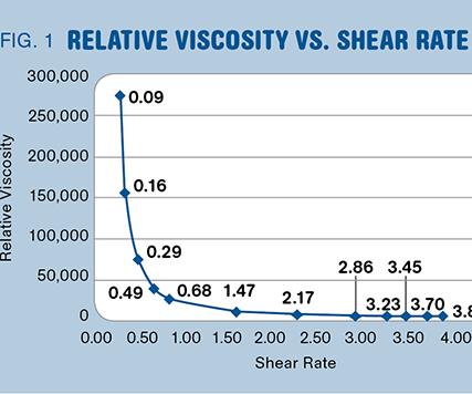
FIG. 1: A typical Relative Viscosity (RV) vs. shear rate curve taught in many training courses for choosing an optimum injection fill time.
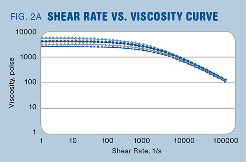
FIGS. 2A, 2B: Resin shear rate vs. viscosity curve from a capillary rheometer resembles the Relative Viscosity curve from molding experiments when converted from the usual log-log chart (2A) to non-log scales (2B).
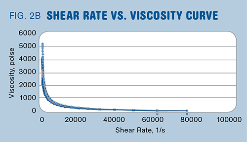
FIGS. 3A, 3B: One problem with the shop-floor Relative Viscosity procedure is that the shape of the curve, and thus the selected optimum fill time, can change if the scale of the graph changes—for example, from carrying out the fill-time tests to 20 sec (3A) or to 5 sec (3B).
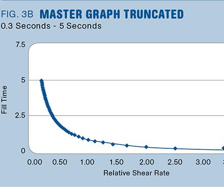
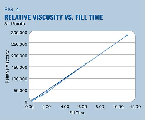
FIG. 4: Graph of Relative Viscosity (RV) vs. Fill Time appears to be a nearly straight line, due to the scale employed.
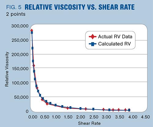
FIG. 5: Fill times from the novel 2 Point Rheology Curve were used to calculate Relative Viscosity and Relative Shear Rate, producing an RV curve nearly identical to the RV curve generated from 12 molding data points. The ability of two fill-time data points to generate the same curves as 12 fill-time points was found to be true for a variety of molds and materials.
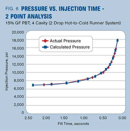
FIG. 6: Back-calculating injection pressure from the 2 Point Rheology Curve gives results very close to the actual pressure in most cases where fill pressure increases with decreasing fill time.
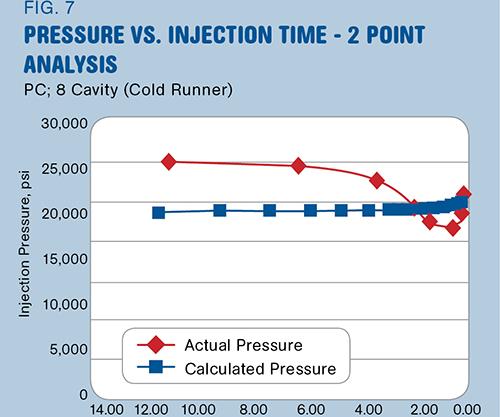
FIG. 7: Injection pressures calculated from the 2 Point Rheology Curve are less accurate when the lowest fill pressure is not at the longest fill time, but somewhere between the fastest and slowest fill, as in this example.
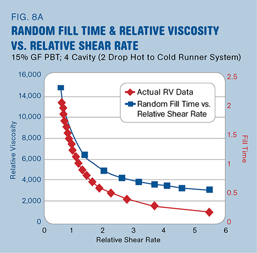
FIGS. 8A, 8B: Plots of RV data were compared with plots of random fill times versus relative shear rate (1/FT) over the same range of fill times used in the actual RV test for the same molds. The resulting two curves are very similar, though the slopes between data points are different due to the influence of pressure on the y-axis values (8A). But when the curves are shifted they overlay on top of one another very well (8B). This was consistent for all molds tested.
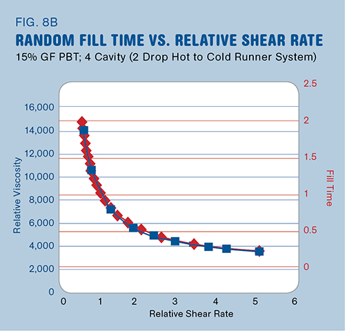
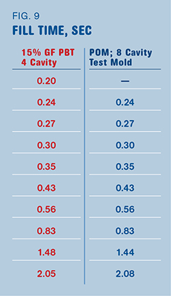
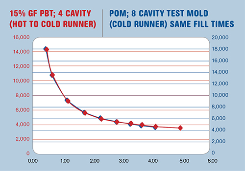
FIG. 9 RV tests were run with acetal in an eight-cavity test mold, but with the same fill times used in RV tests of four other molds with other materials. As shown in this example, those curves in all cases closely matched the original RV curves for the other molds and materials.
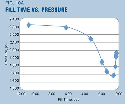
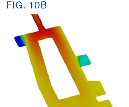
FIGS. 10A, 10B: One avenue of ongoing research into solving the fill-time problem considers the value of the “injection fill-time scan” produced by early versions of mold-filling simulation software (10A). Today, that information can be supplemented with finite-element modeling of melt temperature throughout a mold cavity during fill (10B).


Injection molding process methodologies have evolved over the decades from a seat-of-the-pants black art to a more structured approach. A number of schools, companies, and individuals provide a valuable service to the industry by teaching these structured methods, which have been labeled with terms such as Scientific Molding, Decoupled Molding, and 2-Stage and 3-Stage processes. These approaches involve similar specific procedures that help establish a foundation on which to build a process. Among the procedures taught are a method for determining a fill time or fill speed using in-mold rheology curves (a.k.a “relative viscosity vs. relative shear rate” curves), as well as methods for establishing an ideal transfer position, ensuring the proper melt temperature, finding the ideal hold pressure, identifying pressure losses within the mold, and finding the time when gate seal (gate freeze) occurs.
These approaches also teach that the process must be documented in a manner that allows it to be transferred to other molding machines with the intent of achieving relatively consistent part quality. This requires that the process is recorded by referencing plastic variables, not machine variables, and is done using a “universal setup sheet” (a term used by John Bozzelli, scientificmolding.com). For example, if you are documenting the melt temperature you would document the temperature of the plastic coming out of the machine nozzle—not the barrel temperature settings on the machine controller.
ESTABLISHING OPTIMUM FILL TIME
One of the important process parameters to establish and record for any injection molded part is its injection or fill time. Fill time is an indication of how fast the plastic is injected into the mold. Fill time affects how much shear heating and shear thinning the plastic experiences, which in turn affect the material’s viscosity, the pressure and temperature of the plastic inside the cavities, and the overall part quality (dimensions, aesthetics, strength, etc.). Any change in fill time may adversely affect the final molded part. Therefore once the ideal fill time is established for a given mold, that fill time should live with the mold forever and should be allowed to vary only slightly (±0.04 sec, as per John Bozzelli’s recommendation). The key question is: How does one go about identifying an ideal fill time for a given mold?
Molders use several methods to establish a fill time, some of which begin with one of the following methods:
•Evaluating the fill time used on similar parts and molds.
•Trial and error.
•Design of experiments (DOE) data.
•Experience.
•Mold-filling simulation.
•Relative Viscosity test.
Ideally, every part would be evaluated for fill time using mold-filling simulation performed by a skilled analyst with plastics processing experience. Unfortunately this type of analysis data is not available for many plastic parts, so molders need a method to establish an ideal fill time that they can employ on the shop floor. This is where the Relative Viscosity (RV) test comes into play. The general procedure for this commonly taught method is presented below.
Though some consultants and trainers may add other steps or teach it a bit differently, essentially the approaches are very similar:
1. Using maximum injection velocity, adjust shot size to get the fullest part 95% full.
2. Record the fill time and pressure at transfer.
3. Reduce injection velocity and record the fill time and pressure at transfer.
4. Repeat Step 3 until the fill time is over 10 sec.
5. Use the data to calculate relative shear rates and relative viscosities:
Relative Shear Rate = 1 ÷ fill time
Relative Viscosity = Hydraulic pressure x intensification
ratio x fill time
6. Graph relative viscosity (y-axis) vs. relative shear rate (x-axis).
7. Select a fill time on the “flat” portion of the curve.
The results of one RV test are shown graphically in Fig. 1. Note that the graph is essentially that of “Fill Time vs. 1 ÷ Fill Time” (where the Fill Time on the y-axis is multiplied by its
corresponding pressure). When you graph a number versus its reciprocal, the shape of the curve shown in Fig. 1 is expected. If the change in pressure were directly proportional to the change in fill time, the graph would show a straight line. However, this test demonstrates that as plastic flows faster (higher shear rate), its viscosity is reduced and becomes fairly consistent over a wide range of injection rates.
The RV test results in “viscosity vs. shear rate” curves that look similar to those produced using laboratory capillary rheometers (Figs. 2A, 2B). Figure 2A shows the capillary rheometer data of viscosity (poise) versus shear rate (1/sec) plotted on a log-log graph while Fig. 2B shows the same data plotted on a non-log-log graph. The non-log-log graph in Fig. 2B looks very similar to the RV graph in Fig. 1.
The RV test has been widely taught and adopted by many molding companies to help select a fill time for a given mold. Company procedures have been written to include the test as part of their process standards. Thus, there is a great deal of material, labor, and machine time spent each day on running the RV tests in hopes of identifying optimum fill times based on a structured approach that a process technician or engineer can use on the shop floor.
Ideally, someone applying this technique should also be evaluating the parts for cosmetic issues and other defects to help determine the optimum fill time. But all too often we have found molders looking at the curves as a scientifically founded method to establish optimum fill time and therefore assuming they should look at other process parameters to address molded part problems.
Those who teach the RV test method usually state that for most parts the fill time should be located somewhere on the flatter portion of the curve (after the “elbow”). The flat portion
of the curve is considered desirable because it is expected to produce the most consistent melt conditions when changes occur in the process or resin viscosity. These changes might result from lot-to-lot material variations or process drift.
Depending on the range of fill times used, the flat portion of the curve can be a small area or rather large. This leaves the processor asking, “Where on the flat portion of the RV curve is the optimum fill time?” Currently the practice of picking the fill time from the curve is quite arbitrary. If you ask three different molders taught in the same class to select a fill time from the same RV graph you may get three different answers. Listed below are several common opinions and one formula that have been suggested as guidelines for selecting the target fill time:
Method 1: Halfway from the “knee” to the end of the curve.
Method 2: The point right after the “knee.”
Method 3: The farthest point out, because it has the lowest viscosity overall.
Method 4: ([(Highest RV – Lowest RV) x 0.05] ÷ 2) + Lowest RV.


A further complication is that the selected fill time is completely dependent on the scale of the graph at hand. If the scale of the graph changes (i.e. run the test to only 5 sec instead of 10 or 20 sec), the fill time chosen by using the current visual and arbitrary fill-time selection methods may actually change (Fig. 3A vs. 3B). Also, the ideal fill time may be harder to determine since the flat part of the curve will not look as flat as it does when running the test with more data points at longer fill times.
In addition to some ambiguity in the interpretation of the RV test, the method of focusing on a “relative viscosity” to identify a fill time raises further questions. It was apparent that further research was required to better understand the RV test and determine if it could be improved upon. This research began several years ago and only a portion is reported here.
RESEARCHING THE FILL-TIME PROBLEM
Early stages of this work began with us asking ourselves, “What do relative viscosity and relative shear rate really mean?” The relative shear rate is defined as 1 ÷ fill time, which results in units of 1/sec, the same units used by rheologists for describing shear rates. However actual shear rate depends on the volumetric flow rate, the non-Newtonian characteristics (n), and the specific geometry through which the plastic is flowing, as per the following equation:
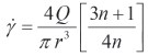
The term relative shear rate differs from actual shear rate in a number of ways. One is that there is no geometry consideration in the relative shear-rate calculation. In actuality, the flow geometry of a mold is constantly changing (nozzle, sprue, progressive runner branches, gates, and cavity). The actual shear rate therefore varies considerably in a mold and can range from a few hundred 1/sec in a cavity to hundreds of thousands in a gate.
During our research we found that when graphing typical RV data vs. Fill time (FT), a nearly straight line developed (Fig. 4). Surely it cannot really be a pure straight line, due to the pseudo-plastic, non-Newtonian behavior of plastics; but the scale at which we are working with causes this to appear linear. From this phenomenon we theorized that we could very closely recreate the original RV curve by utilizing only two data points. This methodology will be referred to as a “2 Point Rheology Curve.”
Utilizing the data from Fig. 4, we selected two random data points. Then we selected a starting (fastest) fill time equal to that of the original mold and increased the fill time by 25% until the ending (slowest) fill time was near that of the original mold. Relative Viscosity and Relative Shear Rate were then back-calculated for the fill times. The result was an RV curve, created using only two data points, that was nearly identical to the original RV curve generated from 12 data points (Fig. 5).
Using the same approach, 2 Point Rheology Curves were then created for more than 40 other randomly selected production molds. These molds ranged from one to 32 cavities; used different melt-delivery systems (hot runner, hot-to-cold runner, and full cold runner); and were run with different plastic materials (such as PP, PC, and glass-filled PBT, PCT, and nylon 66). In each case, the 2 Point Rheology Curve very closely mimicked the original RV curve, similar to Fig. 5.
We theorized that the injection pressure might also be back-calculated for any fill time using the 2 Point Rheology Curve methodology. It was found that this method was within very reasonable limits of calculating fill pressure vs. actual pressure in most cases, regardless of differing cavitation, melt-delivery system, or plastic material. The method was found to provide a good prediction of mold filling pressures in molds where the pressure continually increased with decreasing fill time (Fig. 6 is one example).
In contrast, the method worked poorly in predicting pressures when the lowest fill pressure was not at the slowest fill time, but rather somewhere between the slowest and fastest fill time (Fig. 7). Regardless of the pressure prediction, the calculated RV curves looked nearly identical to the original curves.
Next, the plots of the original RV data for the same molds were compared with plots of random fill times versus relative shear rate (1/FT) over the same range of fill times used in the actual RV test. It was noticed that the resulting two curves looked very similar, though the slopes between data points were different due to the influence of pressure on the y-axis values (Fig. 8A). When the curves were plotted separately and shifted to overlay on top of one another, the two curves overlaid very well (Fig. 8B). This indicates that by using the arbitrary methods of selecting a fill time on a RV curve, it would be nearly impossible to explain why you would pick a different fill time on the original RV curve vs. one from the Random Fill Time curve.
It must be understood that the Random Fill Time Curve data does not include any influence of pressure or material or molding of actual parts. The curve was created by plotting time steps
between the fastest and slowest fill times of the original RV data versus the reciprocals of those time steps. But yet the Random Fill Time curve is nearly identical to the actual RV curve. These findings were consistent over all molds tested and are a result of sound mathematical equations and substitutions.The results prove that any RV curve can be made to look nearly identical to any other simply by adjusting the vertical scales.
Based on these findings and the nature of the RV test itself, we theorized that every mold would produce the same general RV curve, given the same fill times. This would indicate that every mold would have the same selected fill time according to current practices of the RV method.
To test this theory, an RV test was run on an eight-cavity test mold using an acetal resin. The test was performed by strategically changing the machine velocity settings to match the fill times (as closely as possible) to four of the previously tested molds plus the same eight-cavity mold using a PC resin. Thus, five different RV curves were generated for the same eight-cavity mold. Matching the same fill times as the previously tested molds allowed us to maintain the same scale for the Relative Shear Rate x-axis. The data was then overlaid on top of the graph of the original RV data for each of the five molds.
When molding acetal in the eight-cavity test mold, it was found that by matching fill times to those of the original molds, each original RV curve and its corresponding eight-cavity acetal test-mold RV curve looked nearly identical to one another. As an example, Fig. 9 shows the fill times for each mold along with overlaid graphs of the original mold’s RV curve (red) and the eight-cavity acetal RV curve (blue). The x and y-axis labels are removed for clarity reasons but correspond to Relative Shear Rate and Relative Viscosity respectively.
The x-axes are lined up to one another as a result of the corresponding fill times, but as discussed earlier, a shift up/down was required to get the graphs to overlay due to the different slopes between data points resulting from the different pressures required for each material and mold. Regardless, the general shapes of the curves in each figure are nearly identical.
A STARTLING CONCLUSION
The research reported here indicates that if the current practice of using the shape of the RV curve is applied to find a target fill time, it is very likely that the same fill time could be selected for every mold ever made, regardless of material, cavitation, cooling, temperatures, machine, and runner system. The only variation will come from the arbitrarily selected range of fill times that the operator selects to develop the RV curve for a given mold.
The pattern found here may not always be obvious when comparing RV graphs from different molds. The nature of the RV test tends to mask these findings. Consider that each machine and mold combination will influence the range of velocities that can be run during the test. Also consider that each operator will choose different reductions in velocity at each step, and use different ranges of velocity when performing the test. These result in different fill times and pressures, which make each RV curve look different. Essentially the machine/mold and the operator are unknowingly varying the scale of the graph and thereby the appearance of the RV curves.
As it is practiced today, there appears to be little value in performing the RV test as an indicator for determining a fill time when coupled with the arbitrary methods discussed earlier for identifying a fill time. However, one benefit of doing a fill-time scan (versus RV test) would be to see how the mold and part react to different velocities. This will give the operator an idea of what the mold and molded part can tolerate. For example, you may see shear splay near a gate at a higher velocity. This would tell you that you do not want to inject that fast for this particular mold. This would help establish one end (the fast injection-rate limit) of an injection-
time process window. On the other end (the slow injection-rate limit), there may be little reason to run the test up to 10 sec, since most molds have injection times well under that.
You might well ask, “What should we do now to help determine a fill time?” As stated earlier, mold-filling simulation ideally would be utilized, but that simply is not realistic for all molds. So we need an alternative method.
We are studying numerous alternate approaches. One alternative procedure we have worked with has its foundation in mold-filling simulation but is adapted for use on the shop floor. Nearly 30 years ago, injection molding analysts would model an “equivalent rectangle” representing the molded part using a 2D strip file. The thickness of the strip was set to the nominal wall thickness of the part, the flow length was set to the “critical flow length” of the part, and the width would be set as needed so that the volume of the equivalent rectangle would equal the volume of the part.
The analyst would then select a plastic material and a mold and melt temperature and run a series of analyses, each having a different fill time. With early versions of Moldflow software, this was an automated feature referred to as an “injection fill-time scan.” The scan would perform approximately 20 analyses with fill times ranging from very fast to very slow.
The results were presented in a table (and later as graphs), which provided for each fill time a predicted fill pressure, shear rate, shear stress, melt temperature, and cooling time. Of particular interest was the pressure vs. fill time (Fig. 10A) combined with the melt temperature at the gate and at the end of cavity fill. Essentially, this gave the melt-temperature distribution across the cavity, which today we can investigate by plotting temperature from a finite-element model of a mold cavity, as shown in Fig. 10B.
From the tabulated data, the analyst would initially select a fill-time window (range of fill times) where the temperature rise and drop across the cavity was +0° C and -20° C, respectively. Temperature rise across the cavity, resulting from excessively fast filling, was to be avoided because it could complicate packing “far gate” locations. The analyst would then look for the fill times resulting in the lowest pressures, which would often correspond to the region on the bottom of the pressure vs. fill time curve in Fig. 11A. Given these two pieces of information, the analyst would select a target fill-time range based on a condition where melt temperatures across the mold cavity were relatively uniform and pressures were relatively low. It was common that the fill time corresponding to a uniform melt temperature across the cavity would be near to the lowest pressure. It was also considered desirable that the slow end of the target fill-time range be slightly faster than the time corresponding to the lowest pressure, as this would be a shear-dominated rather than thermally dominated cavity condition. This method also has the advantage that it focuses on the part-forming cavity condition, unlike the RV method. Countless molds have been processed with great success utilizing these older simulation techniques.
The fundamentals of the injection-time scan method are quite sound and apply logical methodologies. The process is focused on the quality of the molded part as influenced by the melt conditions within the mold cavity. The currently practiced RV test method is incapable of isolating and evaluating rheological conditions within the cavity. Additionally, the RV data is determined from a conglomeration that includes the energy to move the screw and pressure loss through the machine’s end cap, nozzle, sprue, runner system, gate, and finally the cavity. A stable Relative Viscosity in the overall conglomeration does not necessarily represent a stable viscosity within the mold cavity. It is the conditions within the cavity that are most significant in
determining the outcome of the final molded part.
Unfortunately there is no good technology currently available for the shop floor to determine the melt-temperature distribution across the cavity. However all molding machines have the ability to provide injection pressure vs. fill time data.
Though only being able to evaluate Pressure vs. Fill Time has its limitations, it still can provide molders some valuable information to help them make more informed decisions. Since the user will be focused on the pressure changes instead of a Relative Viscosity number, this methodology will provide a quick indication of the fill time at which the process will be close to being pressure-limited. In addition, we find that “fill time” and “pressure” are terms that a processor is familiar with and are more easily interpreted than Relative Viscosity and Relative Shear Rate. And finally, there are no calculations required for the Pressure versus Fill Time graph other than multiplying your pressure by the machine’s intensification ratio, if needed (not in the case of an electric machine).
Processors, mold designers, and engineers can also be taught how to calculate actual shear rates in selected mold regions. As true shear degradation limits are not well known or understood in this industry, this practice can allow a company to establish a defect log per material and shear rate. This data can be useful to both mold designers and processors. For example, a designer could increase a gate size if the log indicated that the current gate-size and flow-rate combination produced a shear rate that historically caused shear splay for a given material.
We continue to study this approach and teach this information in our continuing education and training courses, along with other methods that could be used to help the molder on the shop floor to identify a preferred fill-time window. These methods include consideration of both fast and relatively slow fill times. If you choose to use the RV method and feel it provides benefit, a great deal of time and money could be saved by adopting our 2 Point Rheology Curve presented here. This data would allow a molder to hone in on the “flat” part of the curve (if desired) much faster and at a reduced cost.
A more recent method we are researching is the concept of a “critical velocity” based on the polymer melt, wall thickness, and flow length. The critical velocity is a condition where the thermal and shear conditions are at equilibrium, establishing relatively stable melt conditions, shear stresses, and frozen-layer thicknesses across the partforming cavity. This method uses our new Therma-flo injection moldability characterization method (see June 2012 issue). The critical velocity would be a material characterization that could provide the optimum fill time for a mold prior to actually running the mold.
No matter which method you choose for finding a fill time, it should be considered only a starting point. The molder should understand the limitations of these methods and adapt the process to achieve the design and application requirements of the actual molded part. This includes consideration of all required quality criteria, including cosmetics, dimensions, warpage, etc. And once the optimum fill time and process have been identified, be sure to document the process using a universal setup sheet.


Related Content

A Simpler Way to Calculate Shot Size vs. Barrel Capacity
Let’s take another look at this seemingly dull but oh-so-crucial topic.
Read More
How to Mount an Injection Mold
Five industry pros with more than 200 years of combined molding experience provide step-by-step best practices on mounting a mold in a horizontal injection molding machine.
Read More
Understanding the ‘Science’ of Color
And as with all sciences, there are fundamentals that must be considered to do color right. Here’s a helpful start.
Read More
How to Stop Flash
Flashing of a part can occur for several reasons—from variations in the process or material to tooling trouble.
Read MoreRead Next

Brand-New Test Method Relates Material, Mold & Machine
It's the first material characterization method developed specifically for evaluating the injection moldability of a plastic melt.
Read More
Troubleshooting Screw and Barrel Wear in Extrusion
Extruder screws and barrels will wear over time. If you are seeing a reduction in specific rate and higher discharge temperatures, wear is the likely culprit.
Read More
Understanding Melting in Single-Screw Extruders
You can better visualize the melting process by “flipping” the observation point so that the barrel appears to be turning clockwise around a stationary screw.
Read More