Published 11/24/2020

The Importance of Gauging Residence-Time Distribution—Part 2

Each molecule in the molded product can have a different residence time. This variance is reflected in the Residence-Time Distribution, which you can learn how to determine below.

Suhas Kulkarni, Fimmtech Inc.

In an experiment, a red-colored pellet was dropped into the machine and the parts were sequentially collected. The color showed up on the third shot and was distributed in the next five shots. For our calculations, we used the number of two-and-a-half shots, since approximately half the part is colored. This shows that the molecules in the one pellet that weighed 0.18 g were now distributed into five shots that collectively weighed 147.51 g. In other words, the introduction of 0.12% additive caused the color distribution over the five shots—indicating pretty effective mixing.

Calculation of the actual residence time is complicated by residence-time distribution.

This also indicates that there are molecules that resided in the barrel for just about two-and-a-half shots and some for about five shots. The cycle time on this part is 25 sec, and therefore a molecule entering the feed throat can be inside the barrel for anywhere between about 62 and 125 sec. So there is a distribution of time, meaning there is no one single time that we can truly consider as the residence time. This range is known as residence-time distribution and is shown pictorially in Fig. 1.

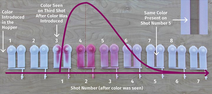
FIG 1 In an experiment, a red pellet was dropped into the machine and the parts were sequentially
collected, with color appearing on the third shot and distributed over the next five.

Same Parts, Same Run, Different Residence Times

The good news is that that this distribution is right-skewed, and most of the molecules are subjected to a residence time on the lower side. The number of molecules on the tail of the distribution curve are significantly lower than at the peak. They are also mixed in with a higher amount of material with lower residence time, which helps maintain properties.

Again, consider the example of the parts discussed in Part 1 of this article, which had a cycle time of 25 sec. If you now take one molded part from the production run, then that part will contain material that had a residence time of 62 sec and a large amount of plastic with a residence time of 75 sec; and over the next three shots there is a tapering down of material with residence times of 100, 125 and 150 sec.

The number 62 is an approximation based on the assumption that half the part has color. There is clearly some material that has no mix of any color in it unlike at the tail of the distribution. The numbers mentioned above are arbitrary numbers picked to represent the local distribution. In reality, it is a continuous distribution, as represented in Fig. 2.

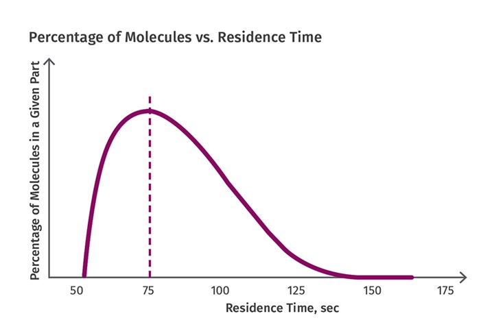
FIG 2 Over a production run, molecules within the parts will experience different amounts of residence time.

The topic of residence time is complicated but must be understood since it plays a critical role in processing. The most common method of calculating residence time is given below in a formula that is effective and practical:

Residence Time = Number of Shots in the Barrel × Cycle Time

where the number of shots in the barrel = maximum machine shot capacity/shot weight.

In the above experiment, the material we used was PS, which has a density of 1.06 g/cc. A machine shot capacity of 100 g would mean that the machine is capable of holding 100 g of PS. However, if the material being molded is PBT, with a density of 1.33, the same volume in the barrel will now have a higher weight. That means the maximum shot capacity in grams of PBT will be higher. Thus,

Shot Size in Material A = (Shot Size in PS ÷ 1.06) × Density of Material A

In case of the PBT it would be :

Shot Size in PBT = (100 ÷ 1.06) × 1.33 = 125.47 g

For all calculations, barrel shot sizes must always be converted into the material that is being molded. Alternatively, the shot weight in the material being molded can be converted into the shot weight in PS.

Accounting for Hot Runners

If the mold in question is furnished with a hot runner, then residence time in the hot-runner system must be added onto the residence time in the barrel. Hot-runner manufacturers can supply the volume of the hot-runner system. Multiplying the volume by the melt density of PS will give the weight of PS in the manifold. The melt density of PS is 0.945 g/cc. Similar to the above calculations, the weight of plastic in the manifold is divided by the shot weight, giving the number of shots in the manifold.

If the info from the hot-runner manufacturer is difficult to acquire, a molder could place just one melt-compatible dark-colored plastic pellet in the machine nozzle-tip orifice and wait to be sure it is molten. With the pellet in place, start molding and count the shots until the first colored parts appear in order to calculate the number of shots in the barrel.

Note: Please exercise extreme caution while undertaking these experiments, including wearing hot gloves, long sleeves, eyewear, and other required safety equipment before performing these studies.

ABOUT THE AUTHOR: Suhas Kulkarni is president of Fimmtech Inc., which specializes in services and training related to plastic injection molding. He earned his Masters in Plastics Engineering from the University of Massachusetts, Lowell, as well as a Bachelors in Polymer Engineering from the University of Poona, India. He has 28 years’ experience as a process engineer and is the author of Robust Process Development and Scientific Molding, published by Hanser Publications, now in its second edition. He also works as a contract faculty member at U.Mass.-Lowell. Contact: suhas@fimmtech.com; fimmtech.com.