
Automate Injection Molding Simulation With Autonomous Optimization
Simulation not only predicts how a mold will fill, but also provides guidance to make it fill better. The new technology of Autonomous Optimization automatically performs hundreds or thousands of simulations, testing multiple variables—gating, venting and cooling, for example—and learning which combinations help achieve objectives for injection pressure, cycle time, warpage, etc.
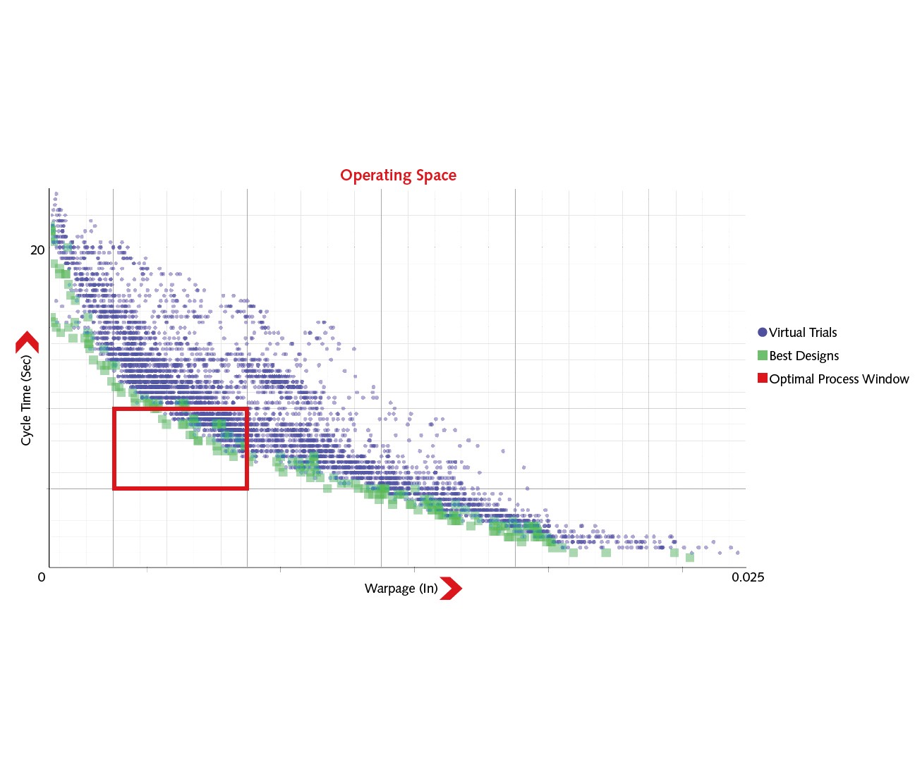
FIG 1 Autonomous Optimization software automatically performs hundreds or thousands of simulations within a predetermined operating space to help find the optimum balance of desired results—in this example, cycle time and warpage.
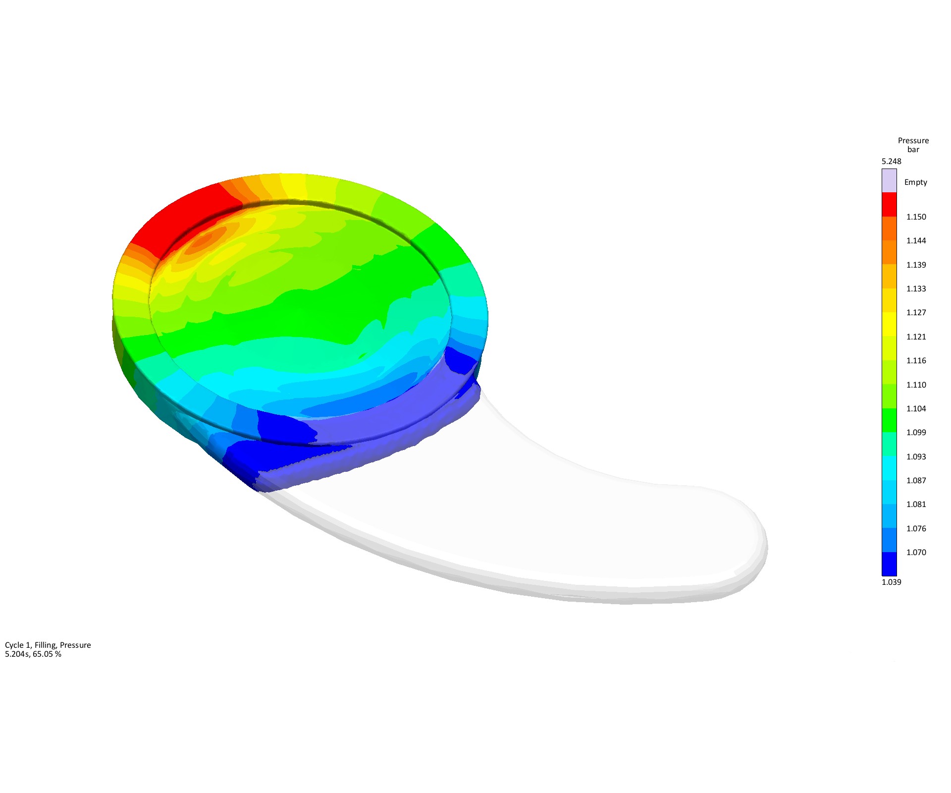
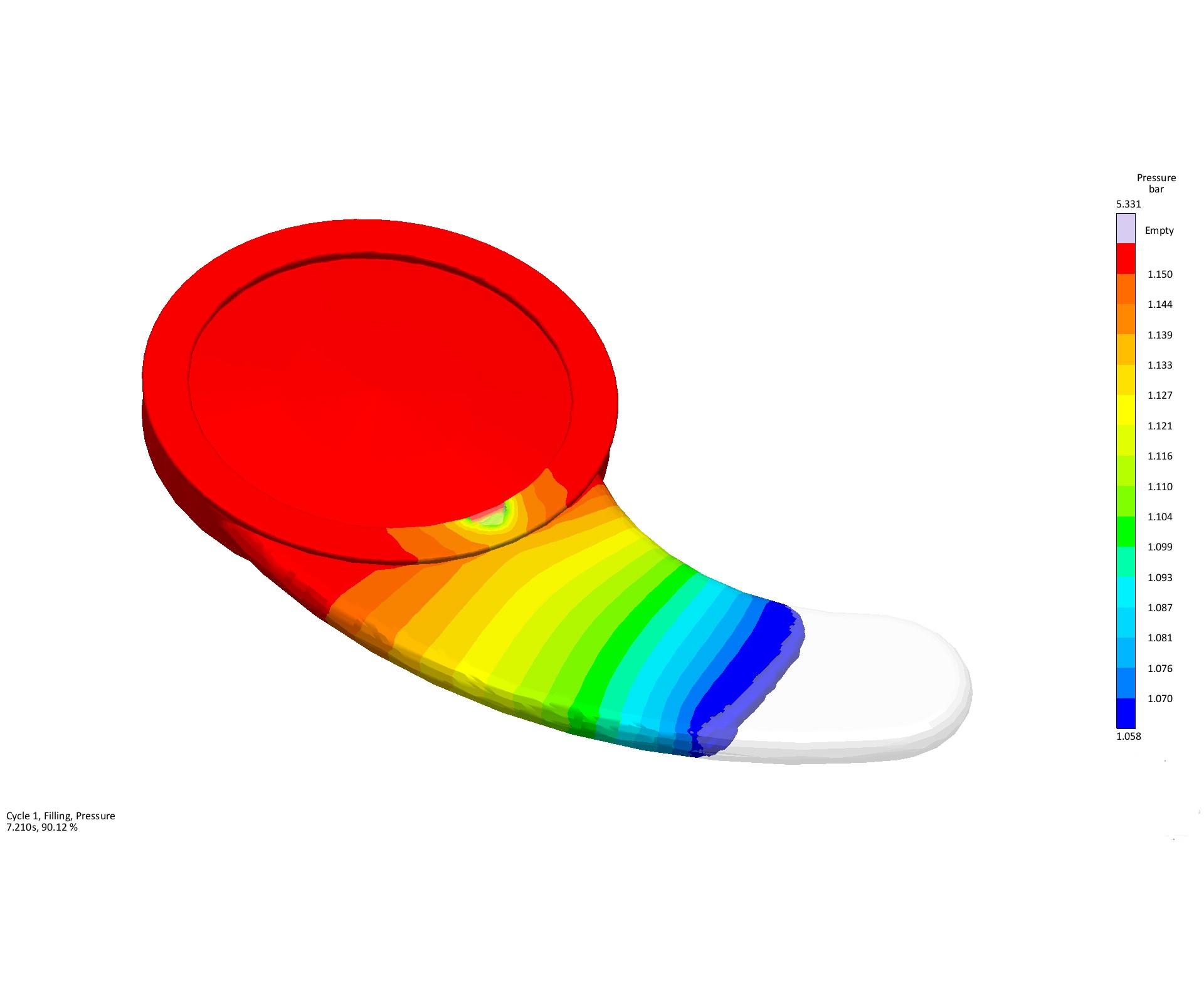
FIGS 2a, 2b In this LSR filling simulation, cavity pressure rises as filling progresses. Air entrapment is forming on the circular rim opposite the gate.
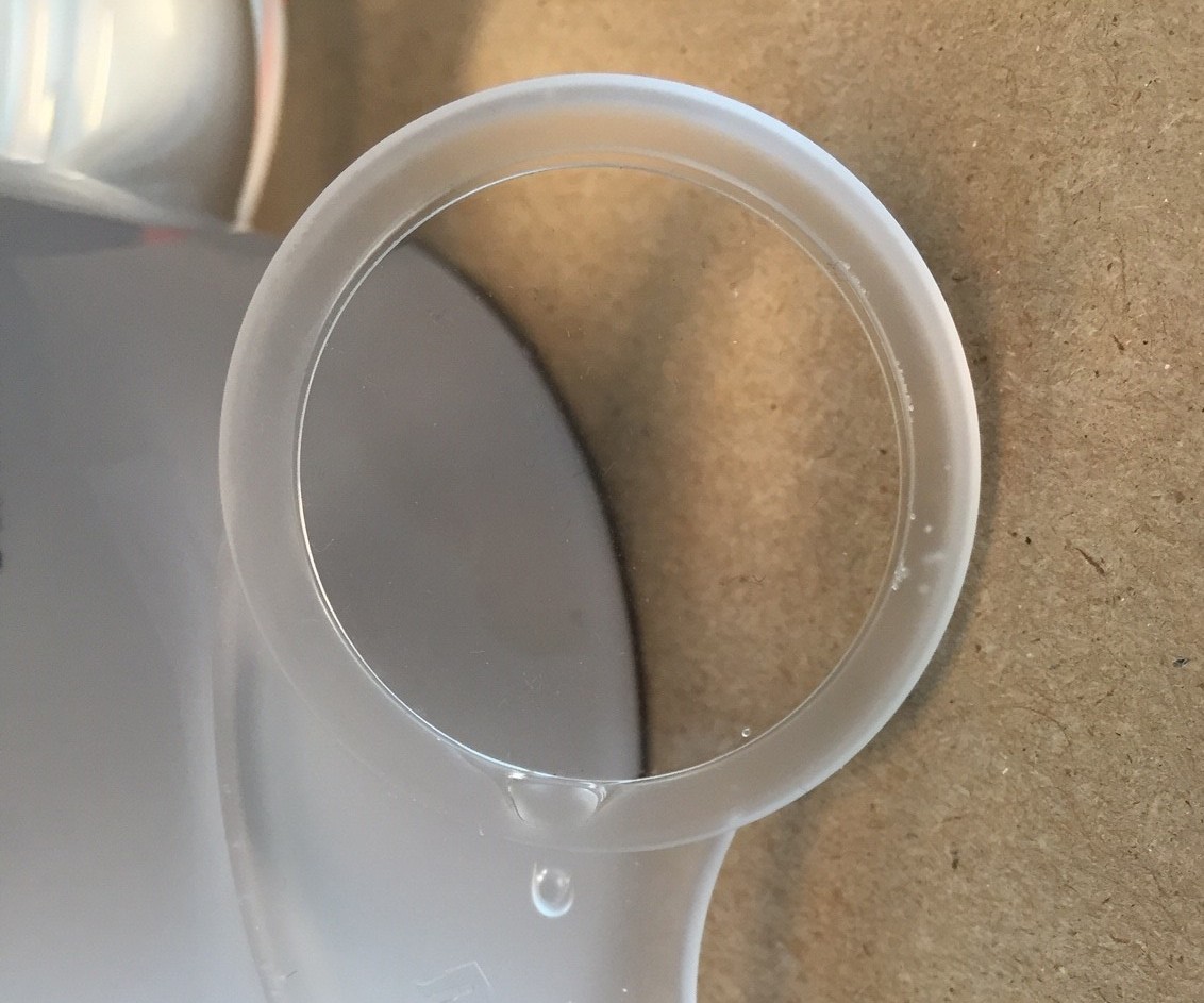
FIGS 3a, b Actual and simulated air entrapment in LSR molding. Bubbles of trapped air (below) are squeezed out of the initial air pocket and into the melt stream. Trapped air can be dissolved in the liquid LSR if the plastic pressure exceeds the trapped air pressure.
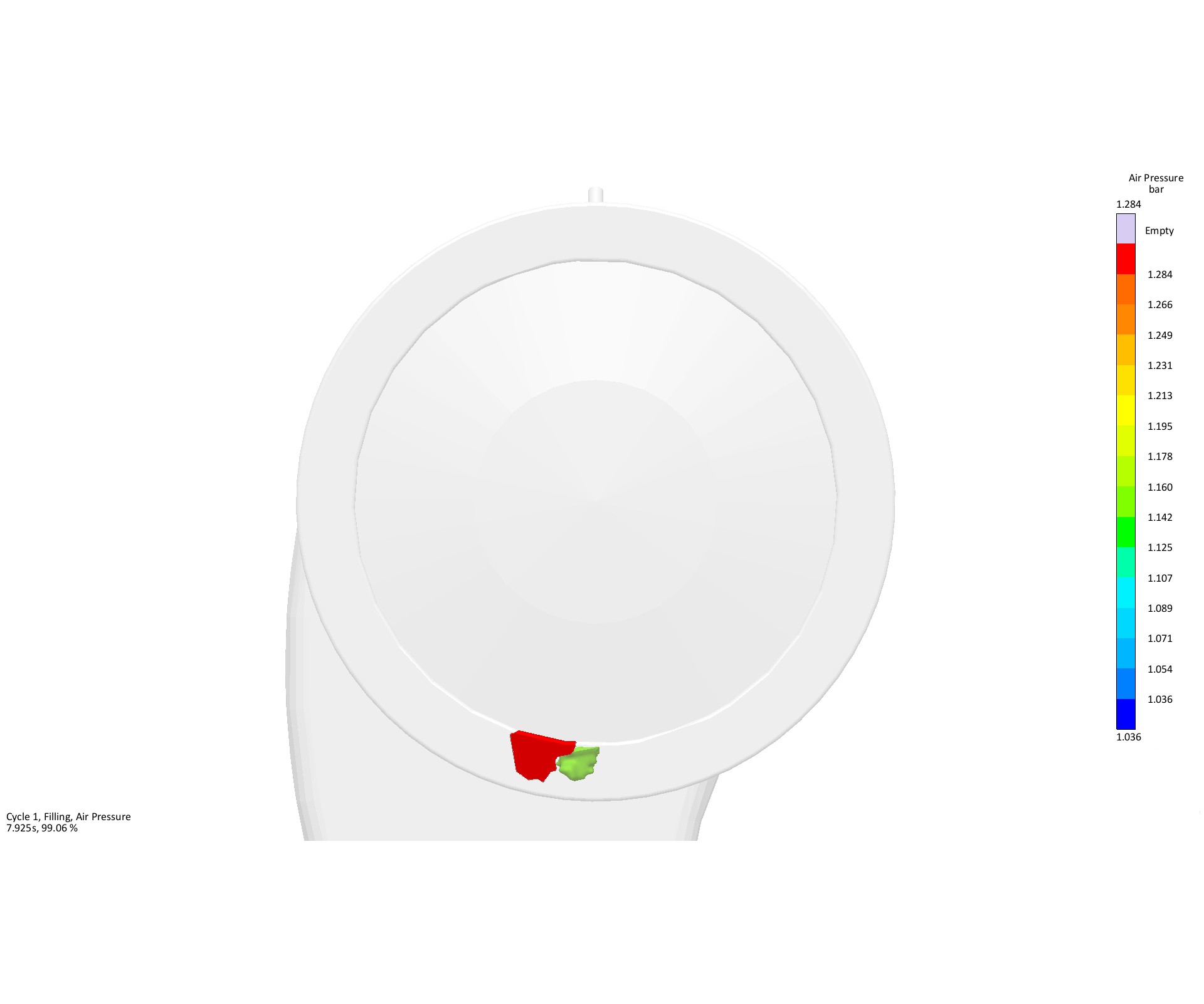
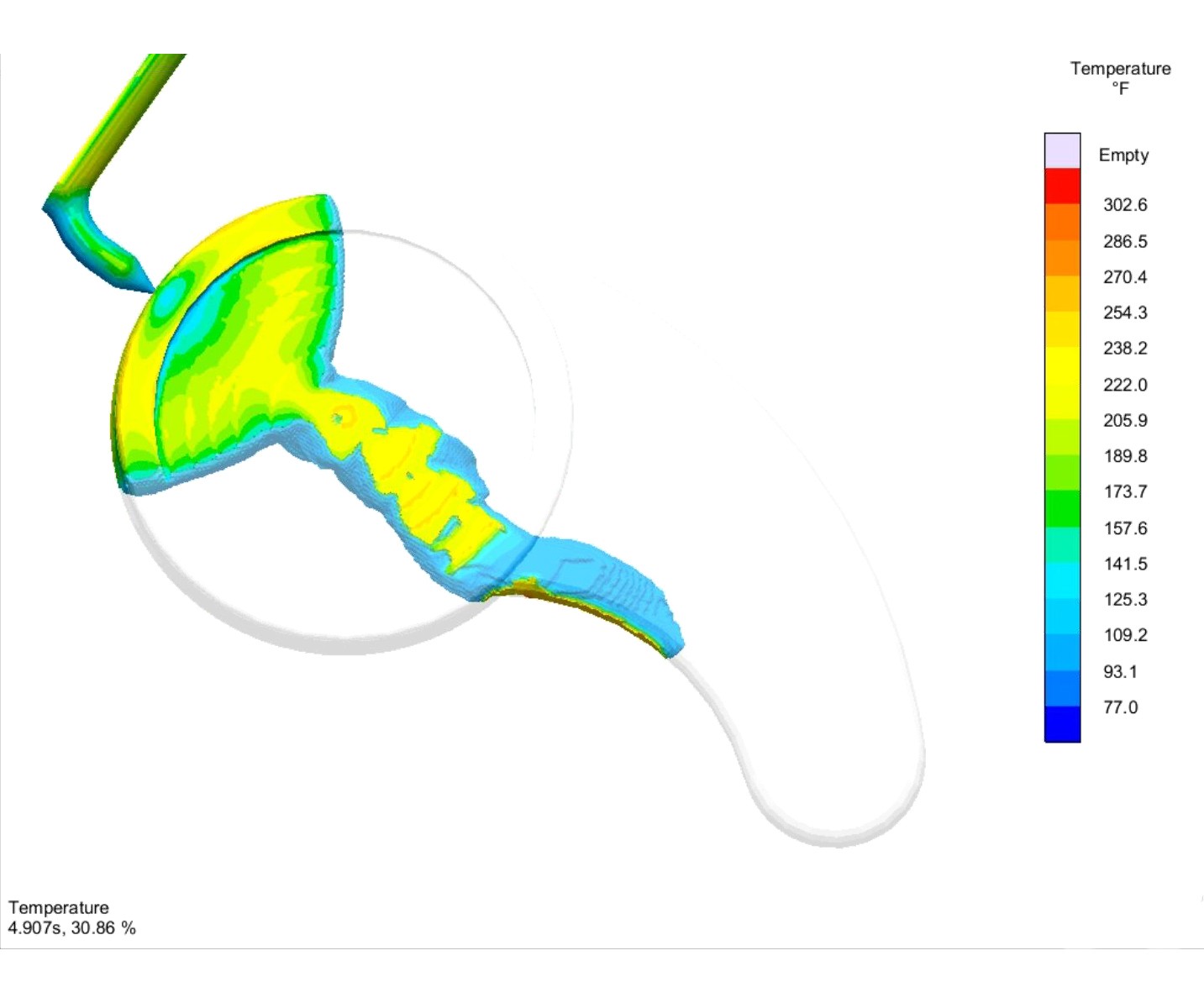
FIG 4 Low-viscosity LSR is susceptible to jetting. Gate location is automatically optimized by assigning an objective of “minimize free surface.”

FIG 5 Possible gate locations are constrained in the software by drawing a dashed line. The software tests 240 gate locations along this arc of 240° and finds potential vent locations based on those gate locations.
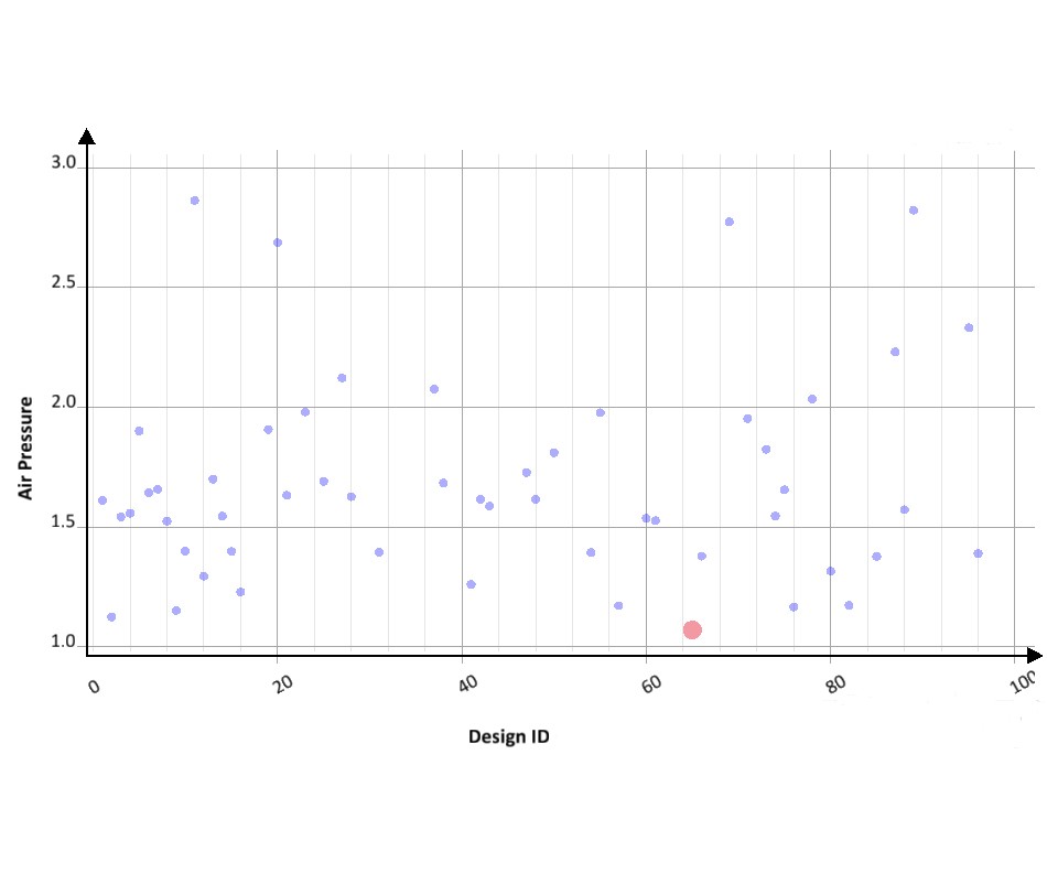
FIG 6 Scatter chart showing each LSR simulation design against the maximum air entrapped. Objectives were to minimize air entrapment by and free surface (jetting), as determined by gate and vent locations. Optimum value is marked in red.

FIG 7a Pressure in the cavity from the original design, showing jetting and air entrapment.
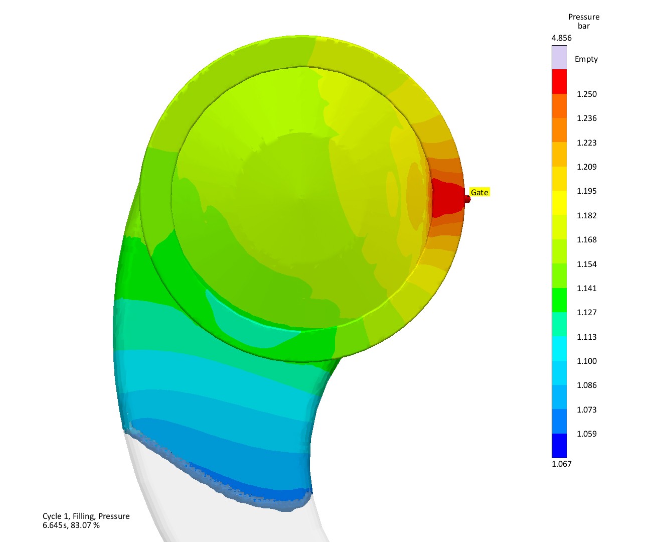
FIG 7b Pressure in the cavity from the best gate location shows no jetting or air entrapment.
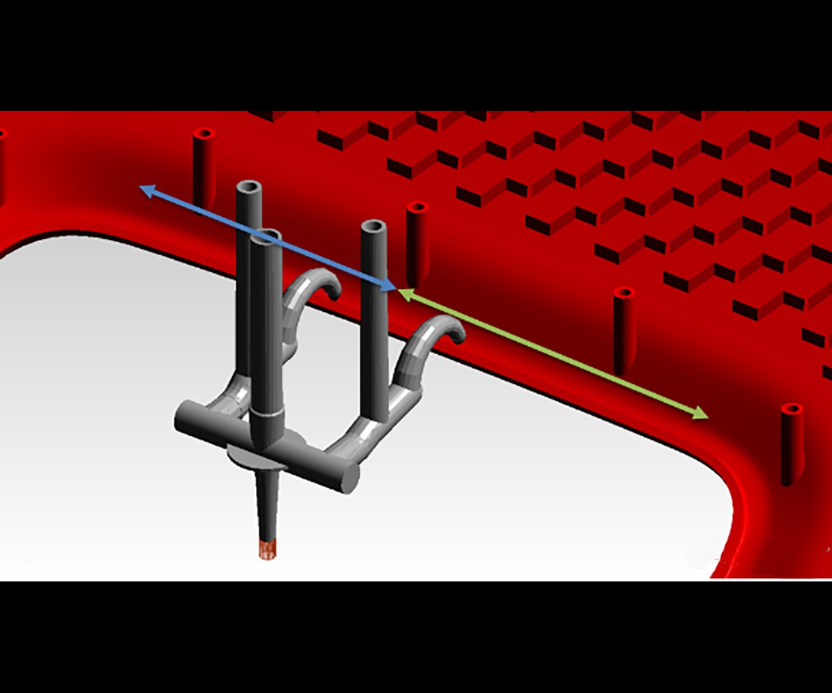
FIG 8 Two gates located in a straight line along an existing rib in a thermoplastic thin-wall part. Paths are shown for permissible locations of each gate along the part.
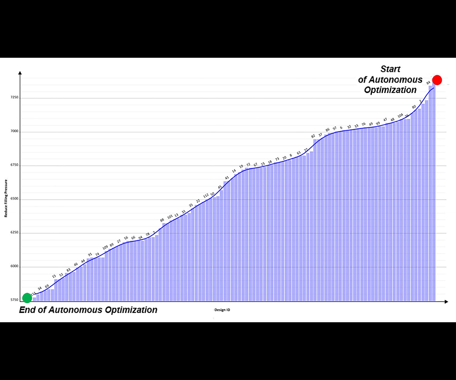
FIG 9 Autonomous optimization of a thermoplastic thin-wall part with the objective of reducing injection pressure. Graph shows the difference in improvement that is possible in 112 variants.
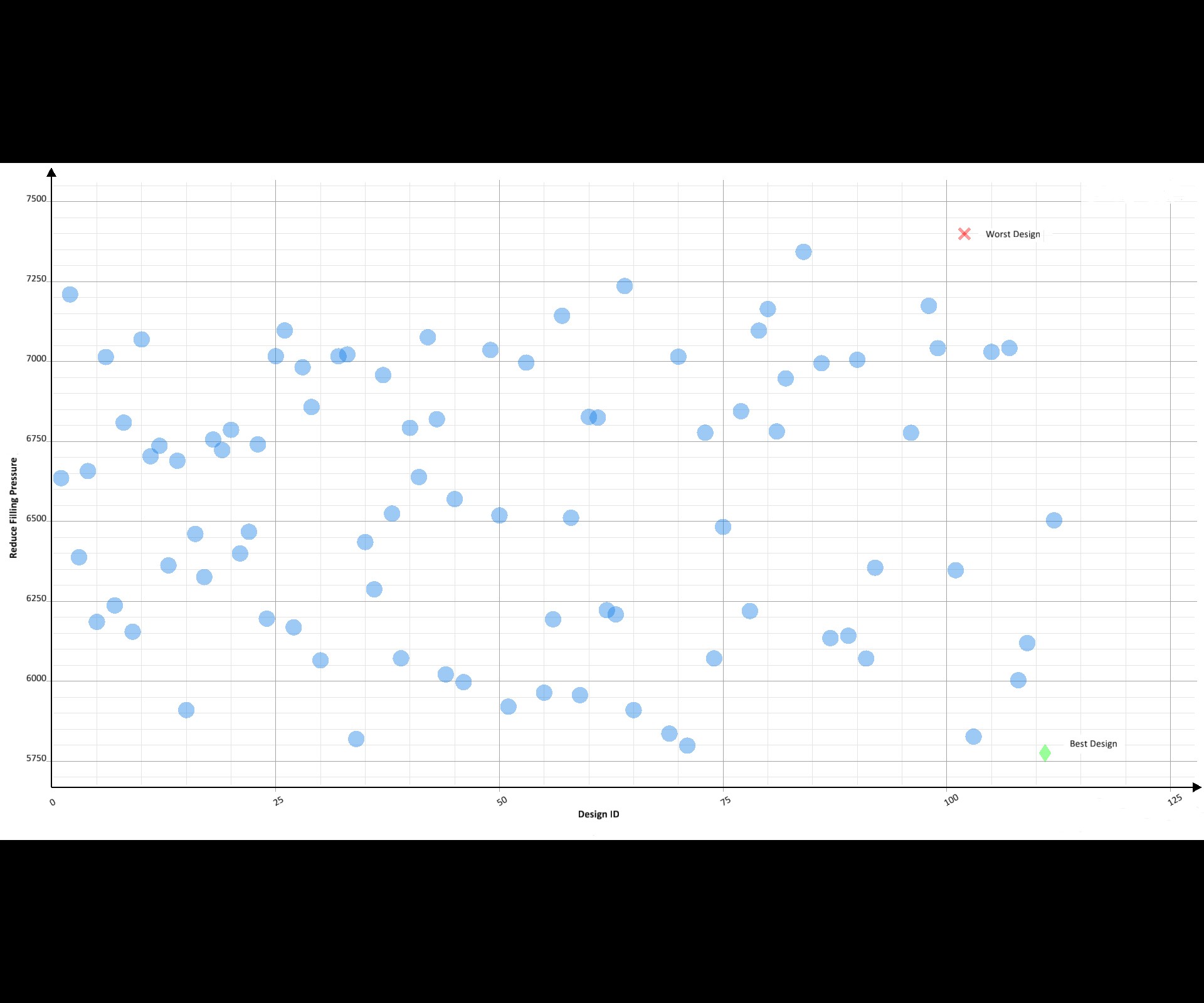
FIG 10 Scatter chart showing same results as in Fig. 9 in a different visualization highlighting best and worst results.
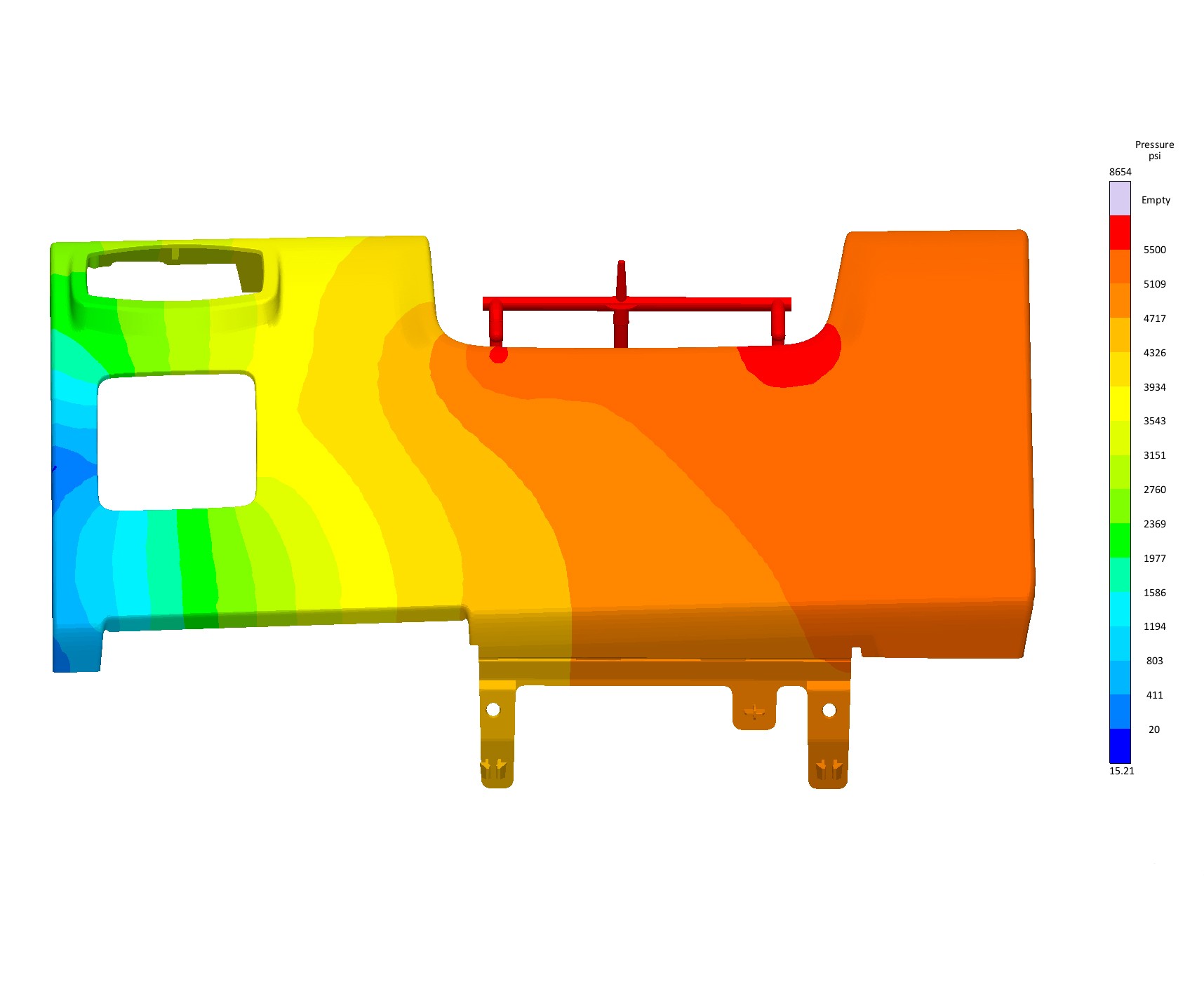
FIG 11a Gate location giving best simulation result from Figs. 9 & 10 with lowest injection pressure.
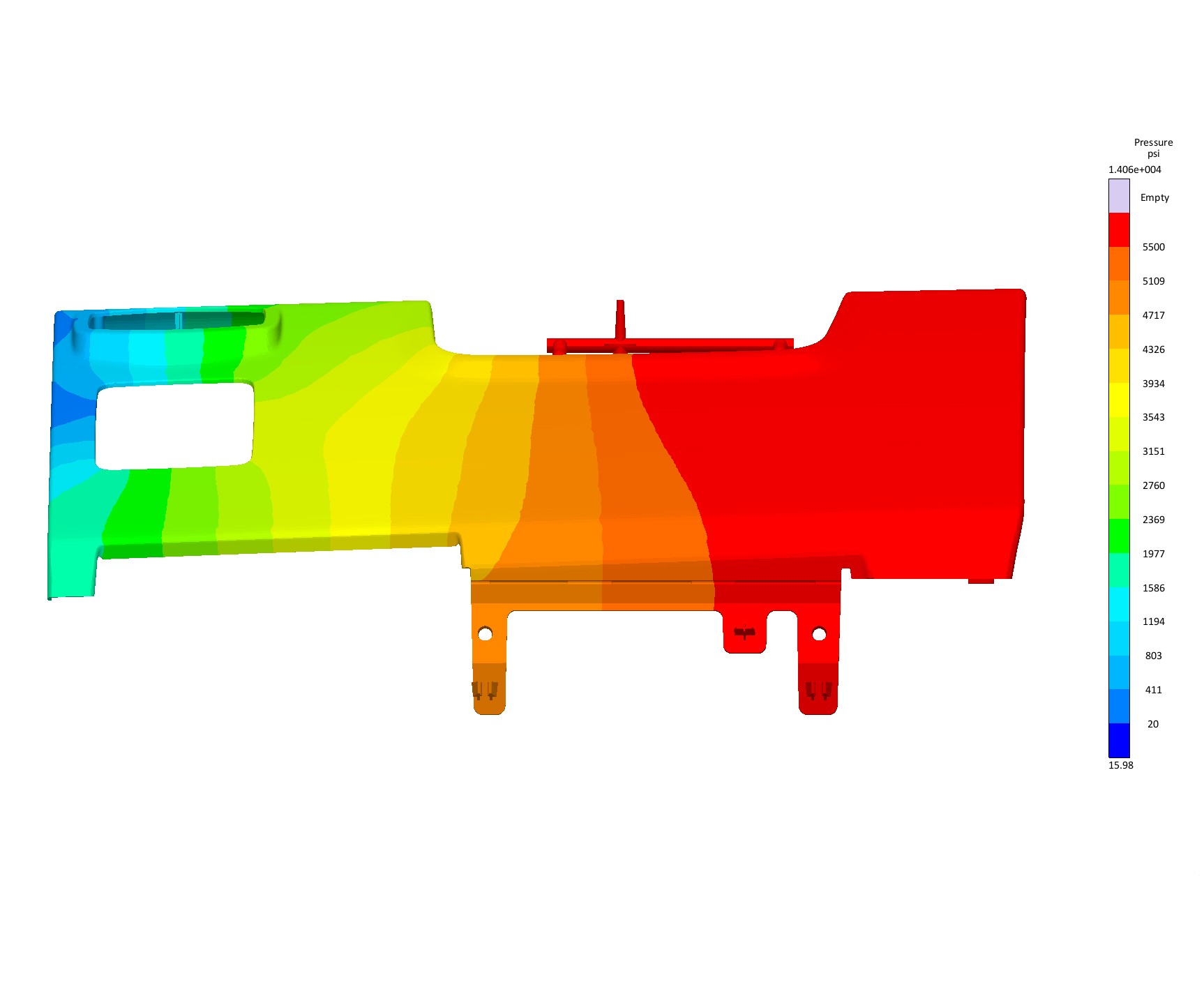
FIG 11b Gate location giving worst simulation result from Figs. 9 & 10 with highest injection pressure.
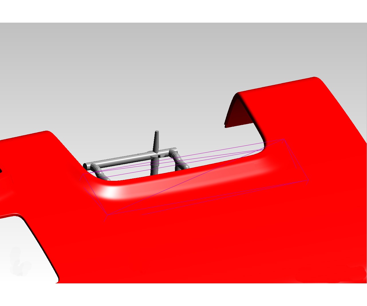
FIG 12 A geometric evaluation area is drawn around the weld-line location between the gates for the objective of reducing weld-line severity.
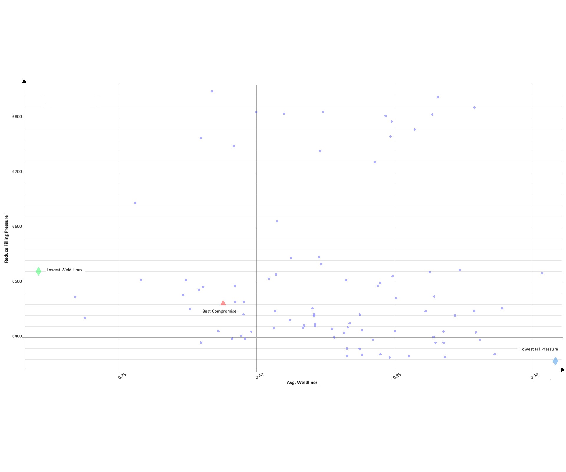
FIG 13 Scatter chart showing best results for filling pressure alone and weld-line severity alone, and the best compromise between the two.
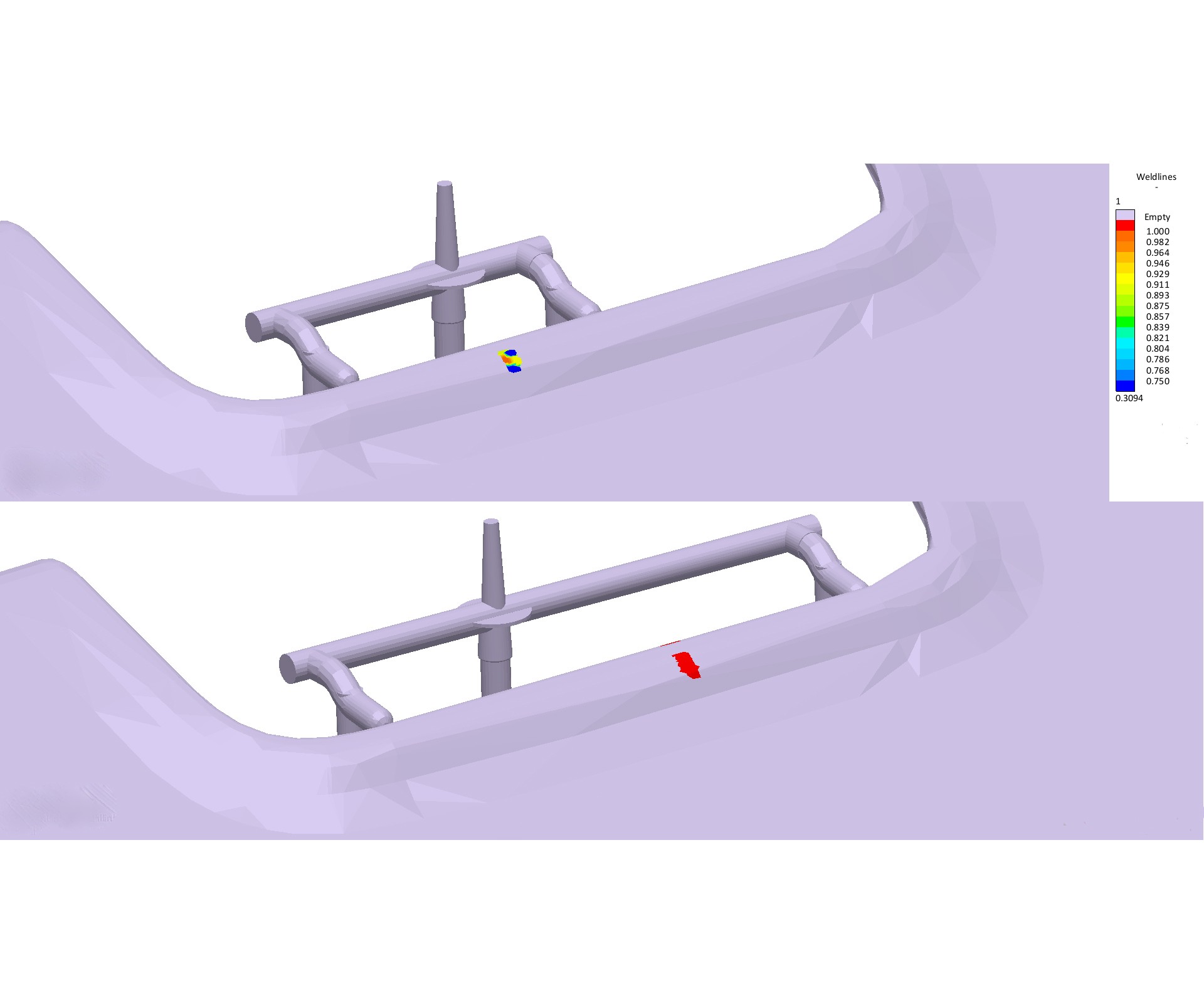
FIG 14 Weld-line severity analysis (higher value indicates a weaker and more visible weld line) for original design (bottom) and optimized design (top).

FIG 15 Cooling layout of a thermoplastic part. Variables for optimizing cooling time are 11 green cooling lines, which can be moved by the software to minimize local mold temperatures.
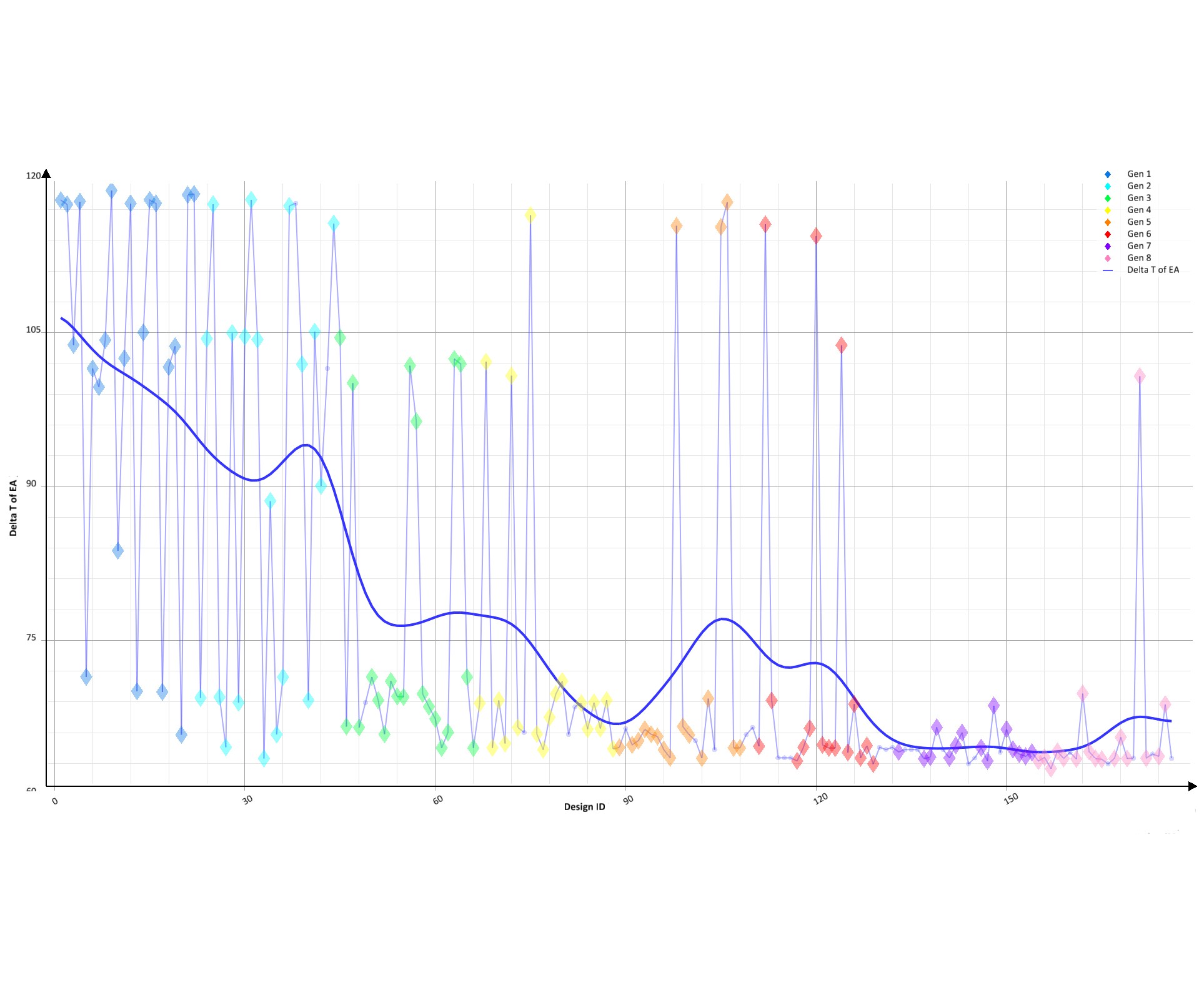
FIG 16 To find the solution that provides the most uniform mold-surface temperature, Autonomous Optimization software used the variables of three mold materials and 11 independent cooling lines, each with from two to seven available positions. The evaluation area for the software was limited to the mold surface in contact with the melt. In just 176 variant simulations—eight generations of 22 designs each—the software learned which variables enable reaching the objective—lowest temperature difference (Delta T) over the evaluation area. The blue line is a smooth curve function of all the data points.
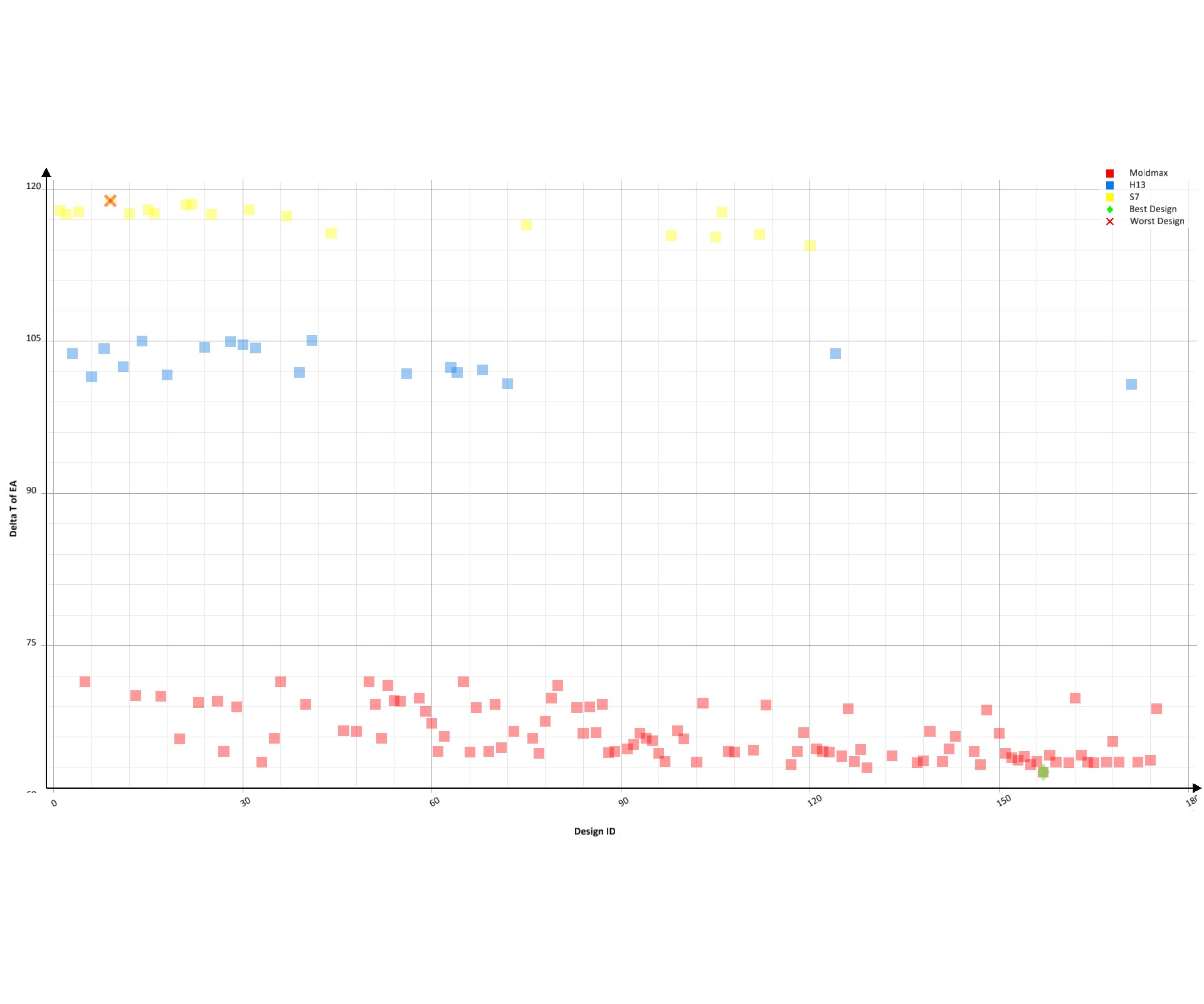
FIG 17 Effect of mold-insert materials. Scatter chart shows mold-surface Delta T for three mold materials and different water-line positions. Moldmax copper alloy yielded the best improvement.
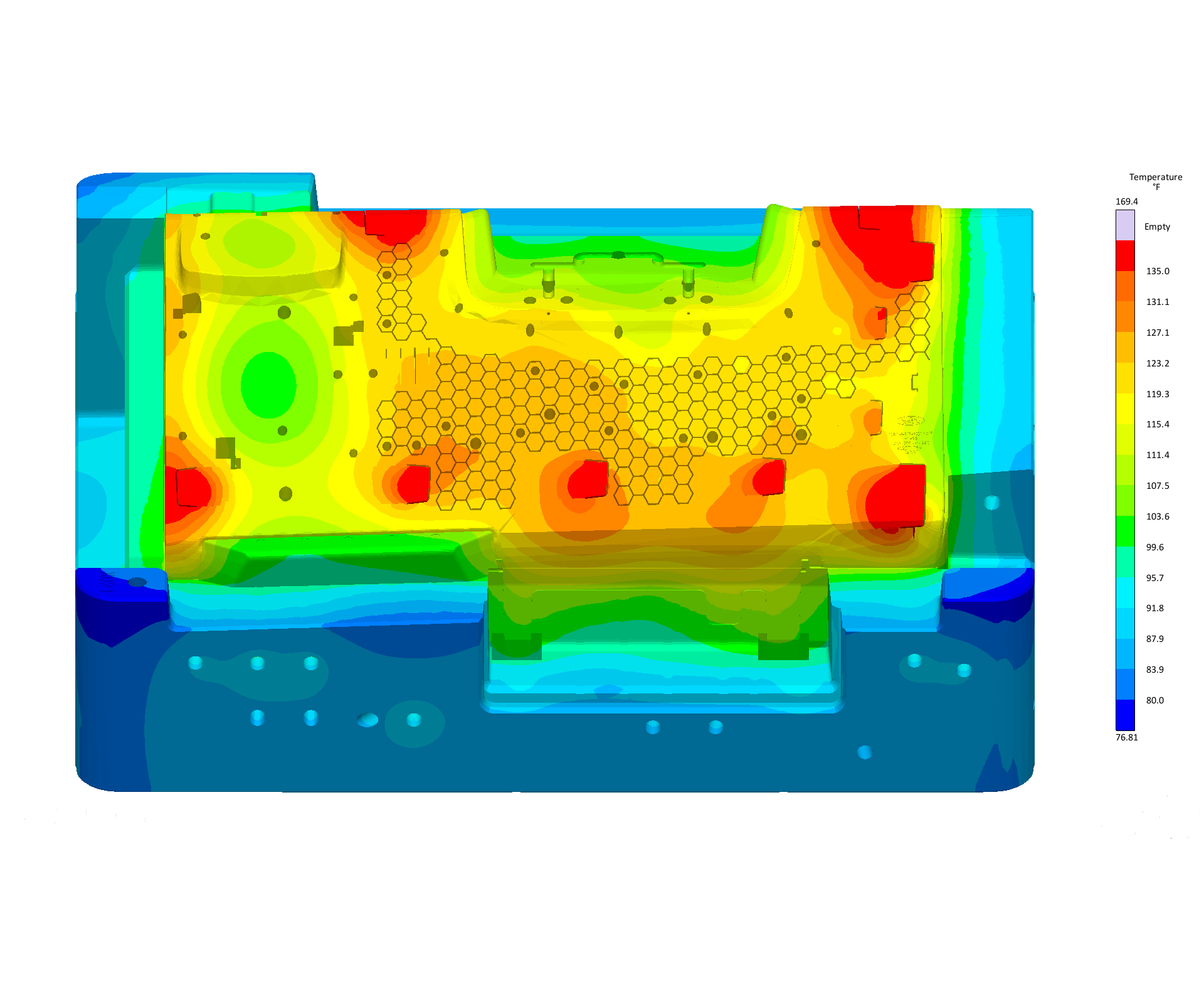
FIG 18a Worst thermal gradient of all the iterations simulated, showing hot spots.
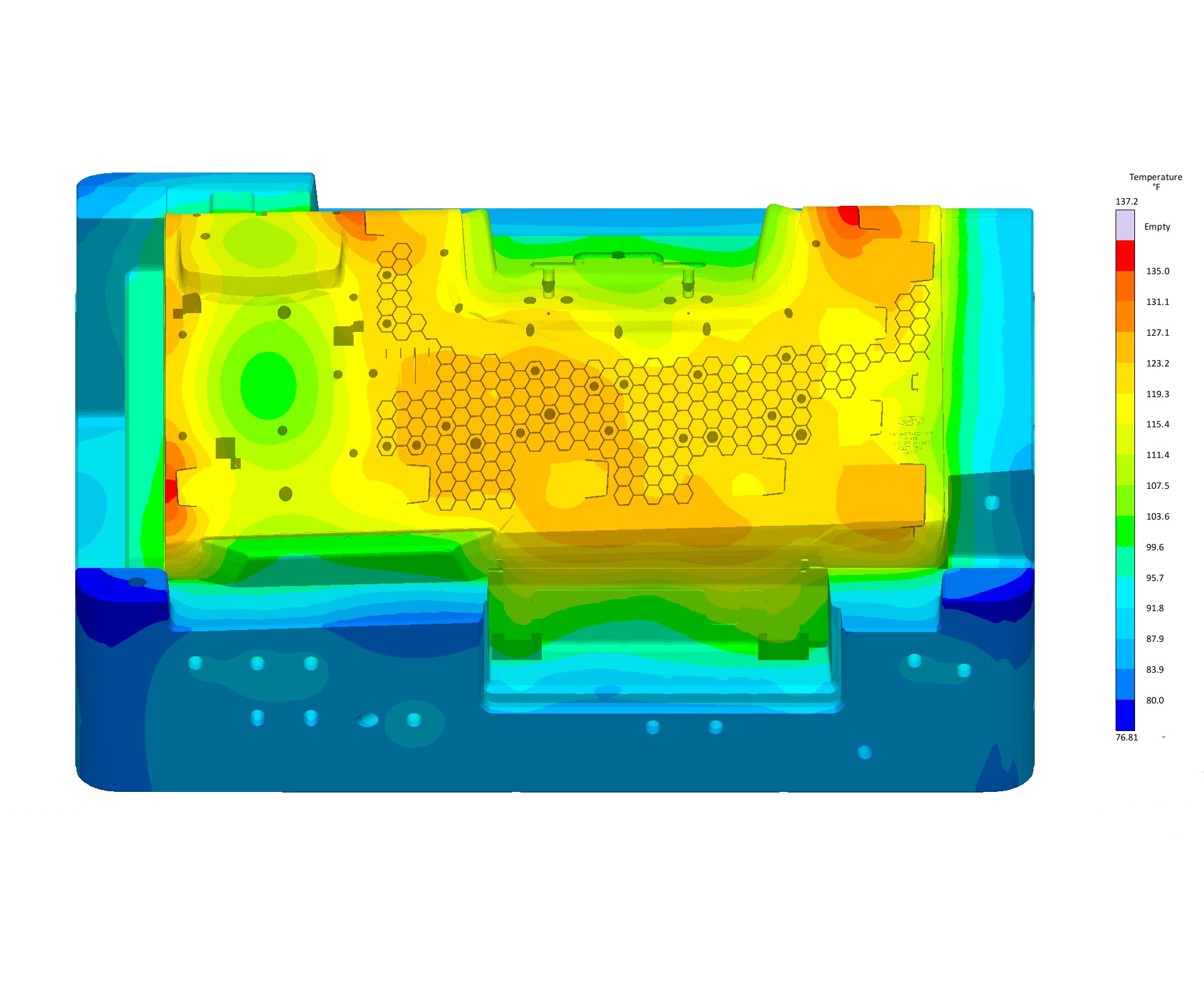
FIG 18b Best thermal gradient of all the iterations simulated, showing elimination of hot spots, whose temperature was reduced from 170 F to 140 F, resulting in a part-temperature reduction at mold open from 300 F to 265 F.
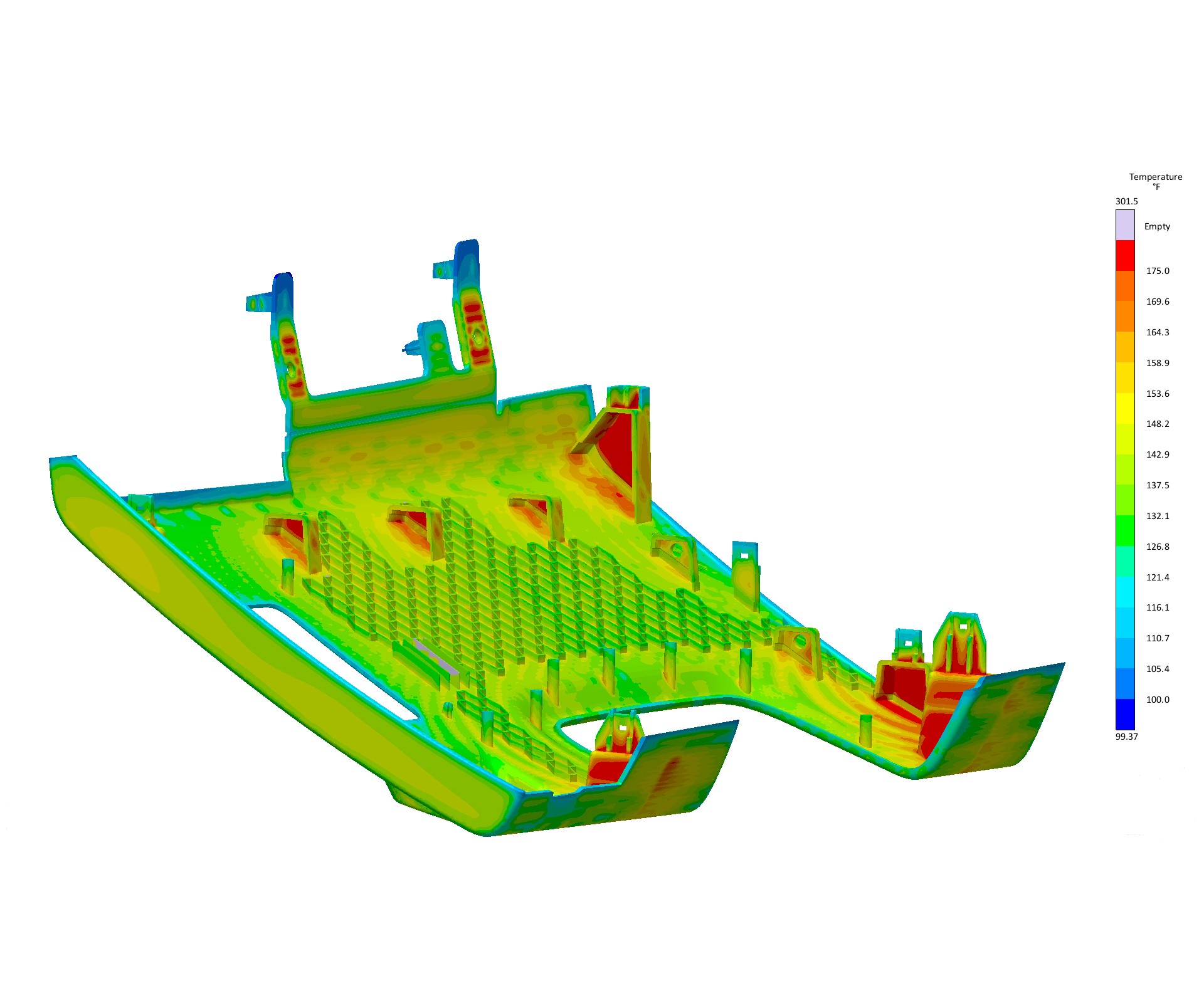
FIG 19a Highest part temperature at ejection—300 F.
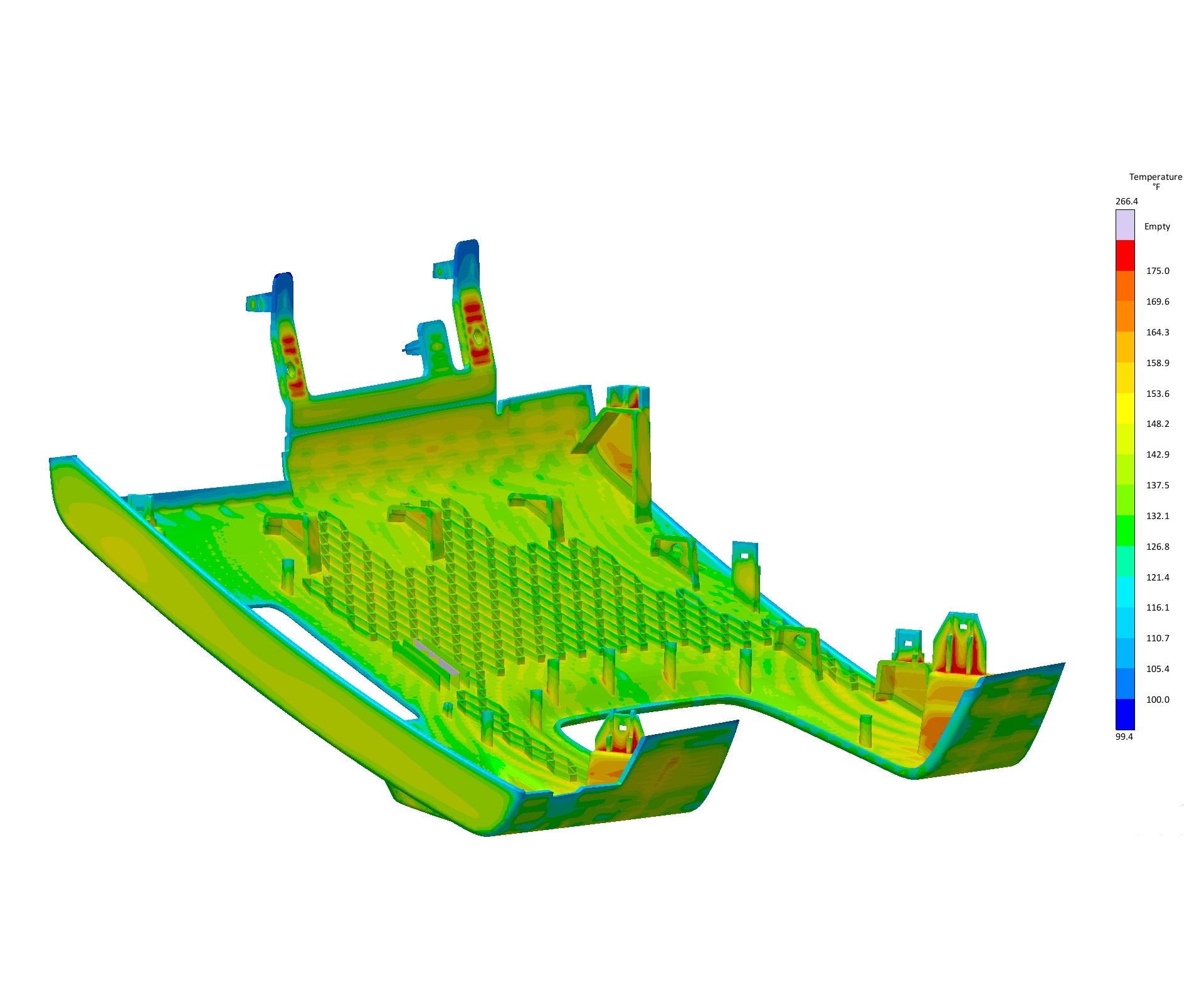
FIG 19b Highest part temperature at ejection (265 F), after elimination of hot spots.
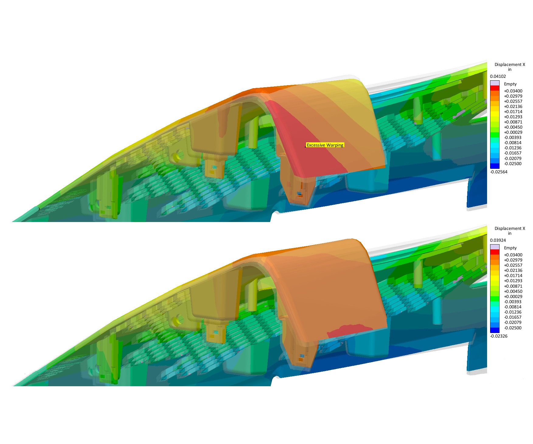
FIG 20 With more uniform mold-surface temperature, warpage is reduced (bottom), even at a faster cycle.


Autonomous optimization is coupled to injection molding simulation to help molders make more informed decisions with less manual labor. The concept is to automatically create and calculate hundreds or thousands of simulations within a predetermined design space of millions of possibilities to learn about the relationship between final part quality and the material, mold, process, and molding machine.
Instead of running 10 simulations with an operator, the software runs hundreds or thousands of simulations on its own. Better decisions are then possible because there is significantly more information to base the decisions on. Obviously, making a decision based on 5000 simulated variations (variants) provides much less room for speculation than basing the same decision on only three or four simulations. With a larger sample size, there is a much clearer understanding of the relationship between the part/mold design and the process. This approach provides even more value to the molder because the software is completing a much larger portion of the work. It’s also completed well in advance of building a mold.


In a traditional simulation approach, an operator sets up a single simulation, clicks start, and then evaluates the results either while the simulation is running or after it’s complete. The evaluation requires time to look at individual results, think about them, decide if improvement is required, decide what inputs to change (probably as a group), make changes, click start, and repeat. This manually iterative procedure continues possibly several times a day for several days until the engineering group is satisfied that the result is as good as it will get with the time available. Each setup might take 15 min and each review might take another 15 to 30 min. Calculation times can vary from as little at 60 sec to as long as an entire day. Manually operating the software for 10 simulation designs can require a full workday of labor, maybe more.
As more data is required for software to make decisions, more simulated variants are required to improve the accuracy of these decisions.
The new, automatic approach is quite different. The software operator sets up the initial design, which includes objectives, variables, and constraints. (This procedure can also be further simplified using pre-existing templates.) The software automatically produces each future variant (simulated design) by changing the process and/or geometry in milliseconds, generates the mesh, queues it up for calculation, runs the simulation, and plots the results of the objectives. The results of all variants are plotted in a single chart so the operator can easily determine which of the variants produce the results that most closely meet their objectives (Figure 1).
The operator time is reduced from 7.5 hr to 0.75 hr (an improvement of 10x). The decisions of the operator are based on thousands of simulations instead of only a few.
This is something like a DoE (design of experiments), which is also possible. However, the main difference is that instead of simulating all of the variants, the software focuses on changes that produce results that more closely meet the objectives. The software knows what can and cannot be changed, how much it can be changed, and what the objectives are, to avoid creating unfeasible situations. It creates and runs multiple variants over several generations, learning about which changes are most desirable. Several variants are calculated in parallel to speed the process. The faster the results are available, the faster the software learns what changes support the desired objectives. This is a completely different approach to solving problems or achieving new goals when compared to traditional simulation.
Making a decision based on 5000 simulated variations provides much less room for speculation than basing the same decision on only three or four simulations.
All molders don’t necessarily have the same goals or constraints. Some may want to find the lowest melt pressure to fit the largest part into the smallest machine while others may want to achieve the fastest cycle time. Some may have significant latitude on gate location or material selection, while others may have none. Autonomous optimization may not be able to find the solution, but it can explore the complete realm of what is allowed to determine the best possible scenario. At least a molder can determine what the very best process is, how repeatable it will be, and what final part quality is attainable.
Two very common problems molders encounter are determining the best gate location and the fastest possible cycle time. But there are other objectives too, all involving part quality. Parts must meet dimensional, aesthetic and mechanical requirements. With autonomous optimization, multiple objectives are used simultaneously to ensure molders don’t end up with undesirable outcomes, such as finding the lowest pressure to fill a cavity but also finding that it creates weak weld lines, or determining the route to the least amount of trapped air but finding that it requires the highest melt pressure.
Automated Optimization software need not perform every possible simulation variant, because it “learns” from each trial which variables lead faster to a defined objective.
OPTIMIZING LSR MOLDING
For LSR production, cavity pressure at the parting line is critical because the material viscosity is typically very low and the material can flash the parting line relatively easily. The pressure rises as the cavity fills, so gate location is directly related to the cavity pressure. Figures 2 a, b show melt pressure rising as cavity filling progresses. The challenge for this product is to determine if there is a geometric solution—i.e., a new gate location—for the trapped air on the circular rim opposite the gate.
The autonomous optimization begins with identification of the objectives, variables, and constraints. Objectives are to minimize air trapped in the cavity during fill. It is described to the software as “minimize: air entrapment” where air entrapment is a specific simulation output. The results are based on the temperature and pressure of trapped air bubbles and are resolved against the liquid melt pressure to calculate if melt pressure rises above the air pressure, it will begin to dissolve into the flowing LSR before curing initiates. Notice the location of the air entrapment and the way in which it becomes trapped (Figs. 3 a, b). Also notice the trapped air bubbles being squeezed out of the initial air pocket and into the melt stream.
The variables in this design will be limited to three—two geometric and one process. Geometric variables are vent locations and gate location. Process variable is filling time at 6 sec and 8 sec.
The two filling times are added to the optimization to make sure the best gate location can also absorb some process variation. Since LSR is susceptible to jetting (Fig. 4) due to its low viscosity, the best gate location must still be valid while being subject to variations in viscosity. This objective is named “minimize: free surface”. Less free surface of the melt will always come from a design with less jetting.
Changes to the vent locations must also be considered (and coupled to the gate locations). This avoids situations where the software finds potentially optimal solutions to the filling pattern but disregards them due to improper venting. The gate locations are also variable, but limited to certain areas of the part. In this case, a trajectory line (path) is extracted from the part geometry and used to keep the definition of where the gate can be (Fig. 5). The gate can move anywhere along the line in 1°. Since the beginning and ending positions of the gate cover 240°, there are 240 different potential gate locations that the software can use to find the optimal gate location. The vent locations are dependent on the gate locations, so additional designs are not required for this variable. Two filling times are combined with 240 different gate locations for a total design space of 480 possible variants. All other inputs for this design were constrained (melt/mold temperature, gate size, material grade, etc.
The autonomous optimization runs multiple designs in parallel for each generation and then runs multiple generations, seeking the gate location that provides the lowest air entrapment within the 6-8 sec range of filling times.
The software has found the best gate location after creating and simulating 96 possibilities. All of the designs are shown in a scatter chart (Fig. 6), plotted against the objectives of lowest air entrapment and least amount of free surface. The best design is identified and exported. The free surface and air entrapment results from the best design are shown and compared with the original design (Figure 7 a, b).
The calculation time for the autonomous optimization was 2 hr and the labor to set it up was only 30 min. In contrast, using a manual approach with both filling times would have taken at least 24 designs to be within 10° of the optimal location. Even at only 20 min (of labor) per design, it would have required a full workday and it would still not be as good as the optimal solution. If it were as good as the optimal, it would have been by accident, whereas the autonomous approach consistently finds more optimal solutions, purposefully, using larger sample sizes and basing decisions on data.
THIN-WALL THERMOPLASTIC OPTIMIZATION
A second example involves a large thin-walled (2 mm), unfilled thermoplastic part where the required injection pressure is forcing the part into a larger machine (or it runs in a smaller machine with an earlier transfer from fill to pack but then forces a struggle to control the shrinkage). The part exhibits excessive warpage even in the larger machine and requires a longer than desired cooling time.
The objective is to reduce the required injection pressure by moving the gates (the variable). This is communicated to the software as: Minimize: melt pressure (@95% filled). On a more complex part design, there can be less flexibility on gate location.
Figure 8 shows that in this case gate locations are restricted to a straight line to keep the gates connected to an existing rib. The blue gate can exist anywhere along its 90-mm-long line (rib) while the green gate can exist anywhere along its own 100-mm-long line (rib). Both can then move in either direction along that rib in increments of 1.25 mm. This results in one gate with 51 possible locations and the other with 61 possible locations, creating a total design space of 3111 possibilities.
The constraints are basically, “Don’t change anything else.” The Autonomous Optimization finishes in 10 hr after running 112 variants. The results show the filling pressure from each design and how each outcome is better than the previous one (Fig. 9).
Autonomous Optimization allows for an efficient and easy way to analyze thousands of designs so a fast decision can be made. Figure 10 shows a scatter chart of the same data as seen in Fig. 9. However, this scatter chart allows for a different visual representation of each design’s performance vs. the desired objective of reducing filling pressure and highlights the best and worst designs. The gate locations that produce the lowest and highest filling pressures are shown in Figs. 11a and 11b.
The new design requires 22% less pressure than the original, allowing it to run in the smaller molding machine. But, there’s a problem: Weld-line results indicate a high degree of severity. This is not acceptable and a compromise must be found. A new objective is created by adding an evaluation area around the weld-line location (Fig. 12).
The new design has two objectives; reduce weld-line severity and reduce required injection pressure, but with the same variables—moving the gates. One can see from the initial results that these might be conflicting goals; gates closer together make for a less visible weld line but gates farther apart require lower injection pressure. The goal is to find the best compromise between the two. The new objective is defined and the existing results from the previous simulations (variants) are reorganized with both objectives in mind (Fig. 13).
It is concluded now that weld-line strength can be improved by 30% (reduced from 100% to below 70%) (Fig. 14) at a cost of only 300psi higher injection pressure, which is still 17% lower than the original. Weld lines are still visible, however. Further reduction in melt pressure is available via gate and runner diameter changes and would be the next step in this new approach.
A gate and runner optimization would be coupled to a viscosity-curve study where the gate and runner diameters would be coupled to different filling speeds to determine the limits of the operating window, thereby saving further time at the molding machine trial.
OPTIMIZING CONFLICTING GOALS
Another common thermoplastic molding challenge is cycle time (specifically cooling time) vs. distortion. These goals are conflicting: Shorter cooling time makes for a hotter part at mold open and likely leads to greater shrinkage outside of the mold (where there is no mold to hold it in shape), which results in a distorted part. A longer cooling time allows the part to cool more inside the mold, where it’s constrained (mostly), holding the part in place until it has higher strength. It shrinks less outside the mold and typically has less distortion. The objective is to find a way to reduce the part temperature at ejection and also reduce the cooling time in the mold.
The variables are the 11 green cooling lines moving independently (Fig. 15). The cooling lines are moving towards the hotspots in the mold in order to reduce the local mold temperature. Mold-steel inserts of three materials—Moldmax high-thermal-conductivity copper alloy (materion.com), H13 steel, and S7 steel—in these locations were considered as another variable. The stated objective for the software is Minimize: part temperature at ejection. Once the best cooling positions are found, the stress calculations for shrinkage and warpage are computed to evaluate the difference between best and initial scenarios.
The first objective is to achieve the most uniform mold-surface temperature (lowest Delta T over that surface area). To perform the optimization, an evaluation area is defined as the mold surface in contact with the melt. There are three mold materials and 11 independent cooling lines with between two and seven available positions, resulting in 3.3 million possibilities. Using Autonomous Optimization with goal-oriented objectives, the complete design space does need to be simulated. The software learns which variables result in reaching the objectives faster. In this case, only 176 calculated variants (eight generations of 22 designs each) were required to find the optimal solution (Fig. 16.).
The cost of multiple automated simulation iterations is much less than the value of the time of a trained simulation software operator.
Figure 17 shows the effect of different mold materials and water-line positions. Moldmax alloy yielded the most uniform mold-surface temperature. The hot spots in the mold reduced their temperature from 170 F to 140 F (Figs. 18a, b), which resulted in a part-temperature reduction at mold open from 300 F to 265 F (Figs. 19a, b). Since the material can be ejected as soon as it reaches 285 F, the results show this occurs at a cooling time of 37 sec compared with the previous time of 42 sec. The stress calculations show reduced distortion at a faster cycle (Fig. 20). The amount of labor required to manually set up, and evaluate 176 variants is estimated at 50 hr, while Autonomous Optimization reduced this to only 4 hr.
The calculation time for multiple simulation iterations is extremely inexpensive compared with the cost of labor; the average hourly cost for software and hardware using a three-year amortization schedule is only $5.00 and it works 24/7. The average hourly cost of a trained software operator is $50.00 (including salary, health insurance, retirement, unemployment, Social Security, etc). So, it makes complete sense to focus on reducing the human labor factor since it’s 10 times greater. It also makes sense to focus on software development that computes more quickly. As more data is required for software to make decisions, more simulated variants are required to improve the accuracy of these decisions.
This approach is statistically proven to find better solutions. Most molders use live molding trials and DoE to make these “data-driven” decisions already. The cost of a live DoE trial (8-hr sample including startup and shutdown—$1000) compared with a virtual molding trial ($50) is much less and will help molders achieve levels of profitability not previously possible.


Related Content

Front-End Mold Simulation Software Simplifies and Streamlines Design
SimForm by Maya HTT highlights its front-end mold simulation software as a solution for mold designers and tooling managers.
Read More
Taking Aim at Warpage With Windage
As a last-gasp attempt to salvage a design prone to warpage, CAE Services has developed a hybrid simulation/real-world methodology to ensure better outcomes for when windage is required.
Read More
Software Suite Creates Integrated Workflows for Optimizing Moldmaking
Eastec 2025: The HxGN Mould and Die Suite includes VISI, WORNC, NCSIMUL and datanomix tools to provide an integrated workflow from design/engineering to manufacturing and automation.
Read MoreRead Next

For PLASTICS' CEO Seaholm, NPE to Shine Light on Sustainability Successes
With advocacy, communication and sustainability as three main pillars, Seaholm leads a trade association to NPE that ‘is more active today than we have ever been.’
Read More
Lead the Conversation, Change the Conversation
Coverage of single-use plastics can be both misleading and demoralizing. Here are 10 tips for changing the perception of the plastics industry at your company and in your community.
Read More