
Brand-New Test Method Relates Material, Mold & Machine
It's the first material characterization method developed specifically for evaluating the injection moldability of a plastic melt.
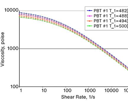
Fig. 1: Characteristic log-log plot of viscosity vs. shear rate and temperature for a non-Newtonian plastic melt.
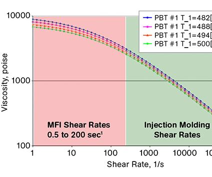
Fig. 2: Viscosity vs. shear-rate graph contrasting the shear rates experienced during a MFI test with those found during injection molding. The pink region is common to materials with MFI under 100. The green region is the higher shear rates found in injection molding.
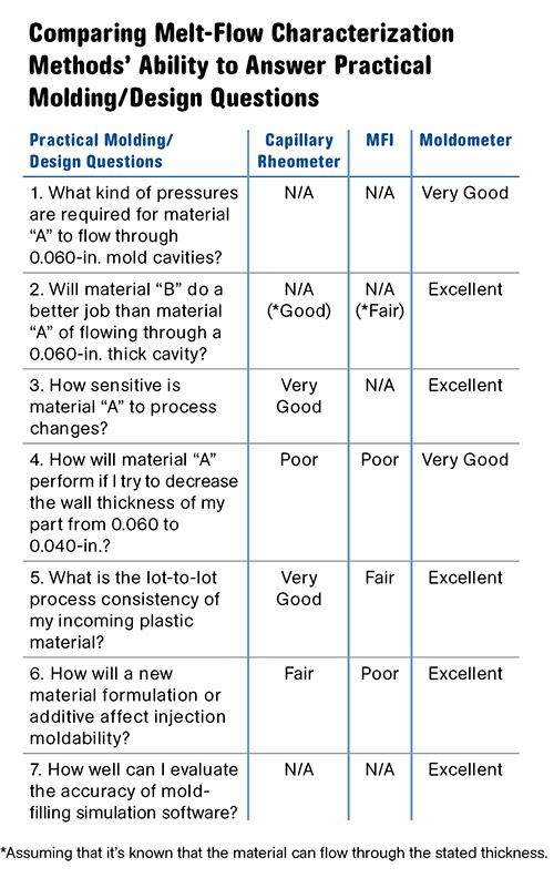
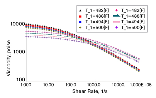
Fig. 4: Viscosity vs. shear-rate curves of two PBTs having different MFI. The lower-MFI (higher-viscosity) material actually has a lower viscosity at the higher shear range found in injection molding.
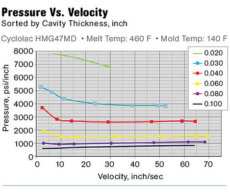
Fig. 5: A Therma-flo Moldometer data sheet of an ABS material developed for Nexeo Solutions. The data sheet includes both cavity and runner information.
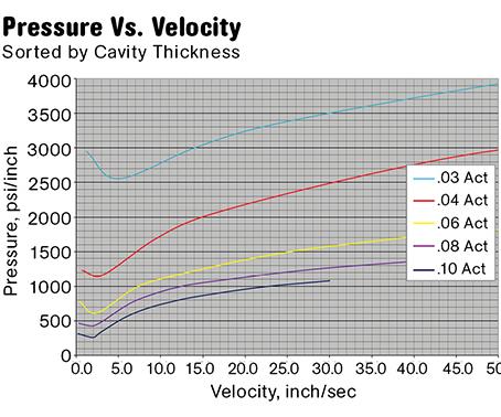
Fig. 6: Therma-flo Moldometer cavity analysis of a HDPE.
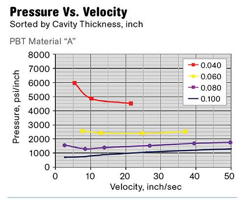
Fig. 7: Therma-flo Moldometer cavity data for two PBTs whose only difference is their additives. Note the different behavior at the thinner wall sections.
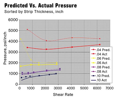
Fig. 8: Veri-flo data contrasting actual molding conditions using the moldometer with injection molding simulation predictions. Note that simulation errors at low shear rates can be accounted for by the analyst.


"Can I mold that part with this material in this machine?" It’s perhaps the oldest question in injection molding, and now there’s a way to answer it with more practically relevant data than ever before.
Mold designers, part designers and processors commonly rely on melt flow index (MFI) data as an indicator of how a plastic material will process in an injection mold. This is often the only data available for a mold or part designer to make critical decisions such as estimation of whether a mold can be filled, selection of gating locations, sizing of runners and gates, or determining cavity wall thickness. The problem is that MFI data is generally a very poor indicator of how a melt will flow through a mold and often results in bad decisions.


It is generally expected that a high-MFI melt should be easier to mold than one with a low MFI. But how often have you selected a material based on this type of data, only to find that it had little or no relationship to how the material actually processed?
Unfortunately, one might find that an 8 MFI nylon fills a mold with less pressure than a 20 MFI nylon (opposite to what is indicated by the MFI data). Or one PBT fills a mold much easier than a second PBT with the same MFI. And a MFI of 12 means something completely different for a nylon than it does for a PC or a PMMA or a HDPE. Did you ever wonder why?
In response to a growing need for plastic melt characterization for injection molding, Beaumont Technologies has developed its patent-pending “Therma-flo” Moldometer. This new method characterizes the injection moldability of a plastic material through a broad range of mold geometries and processes using an actual injection molding machine. The new method significantly improves on the ability of a mold or part designer to make informed decisions when selecting or designing for a given plastic material. It also helps the injection molder to determine whether a particular machine will be capable of filling that mold.
During the plastic material selection process, one must consider both the application and the manufacturability requirements of a material. One of the more critical considerations when selecting a plastic material for manufacturability is trying to determine how it will flow in an injection mold. I refer to this as “injection moldability.” Before delving into the various factors comprising injection moldability, let’s review what happens as a plastic melt flows through the sprue, runners, gates, and cavities of an injection mold.
WHAT THE MELT SEES IN MOLDING
The injection mold-filling process is highly complex and often not fully understood. First, we are trying to deal with a heated non-Newtonian fluid (plastic melt) with a thermally sensitive viscosity flowing through relatively cold mold channels with varying cross sections. Second, the actual melt temperature of these thermally sensitive materials is dependent on a thermal balance between heat loss through conduction to the mold and heat gained from viscous dissipation (shear). And third, there are freezing flow boundaries (frozen layer), which cause the actual cross-sectional size of the melt-flow channels (sprue, runner, gates, and cavity) to be continually changing.
The challenge is exacerbated by the fact that plastic melts have a relatively high viscosity, which requires filling pressures that can exceed 30,000 psi. Higher and higher pressure limits of molds and machines are continually being challenged by part designers who seek to use higher-molecular-weight materials for improved end-use performance and thinner cavity walls to reduce part cost and weight.
Currently there are three primary methods for evaluating plastic flow behavior in a mold. Why aren’t they sufficient to accomplish this task? Let’s look more closely at each of these different techniques.
CAPILLARY RHEOMETER
The first method is a capillary rheometer. This isothermal extrusion test is probably the most detailed means of characterizing a plastic melt. With this method, you can look at the viscosity versus shear rate of a non-Newtonian fluid while also looking at the effect of temperature on viscosity.
A capillary rheometer consists of a heated chamber that is loaded with plastic pellets that are manually compacted and heat soaked until the material becomes liquid. A ram is then driven forward at controlled velocities utilizing a computer-controlled drive mechanism. This forces the melt through the heated chamber and down through a small capillary (commonly 1 mm diam.). Ram velocities are progressively increased or decreased to get multiple shear rates while pressure is normally measured just prior to the capillary with a direct melt-pressure transducer. From the ram displacement, the flow rate through the capillary can be determined.
The next steps include calculating apparent wall shear stress and apparent wall shear rate through the capillary, from which viscosity is determined. After this, Bagley and Rabinowitsch corrections must be applied. The Bagley correction requires a second capillary rheometer test to account for the fact that pressures are measured prior to the melt entering the small capillary.
Once data is collected from a capillary rheometer, it’s typically represented on a log-log graph (see Fig. 1). On the “Y” axis is viscosity, with units commonly represented in poise, Pascal-seconds or psi-seconds. On the “X” axis are shear rates expressed as reciprocal seconds (1/sec or sec-1).
This test method provides detailed knowledge of how the melt’s viscosity behaves under a wide range of shear rates and how it reacts to temperature changes. By itself, this information and its units are fairly abstract and rarely used directly by anyone outside of polymer testing labs or polymer compounders.
The primary use of this data is for injection molding simulation programs. These programs are designed to take this isothermal test data and couple it with thermal solutions to predict how melt will flow through a mold. Without the simulation, the capillary rheometer data has little use in the process of selecting plastic materials for an application by a designer or processor. It is only through use with simulation software that this data can be used to provide meaningful information.
MELT FLOW INDEX
The second method is melt flow index (MFI), which is by far the most common method used for characterizing plastic materials due to simplicity and low cost. It’s interesting that injection molders, practitioners of one of the most complex mainstream manufacturing methods in existence, settle for simplicity and low cost as their primary means of guidance, particularly when the conditions of this isothermal extrusion method are so unlike injection molding.
Unlike a rheometer, which is used to characterize the viscosity behavior of a non-Newtonian melt at multiple shear rates, the MFI test is used to develop a single reference value. Like the rheometer, this is also an isothermal extrusion test; and, as defined by ASTM D1238, it is somewhat similar to a capillary rheometer.
The test begins by hand-loading plastic pellets into a heated chamber. They are compacted and heat soaked until they reach a desired temperature and then a load is applied to a piston to drive the melt through a small orifice. Once the load is applied, the melt will extrude out through the small orifice in the bottom, collecting in a sample container. Over a period of 10 minutes, this material is collected and weighed. The result is a single MFI data point expressed in grams per 10 minutes.
In contrast to the capillary rheometer, not only is only one data point collected but the speed (velocity) of the ram injecting the material through the small orifice is not controlled. Therefore each material having a different MFI will have been measured at a different shear rate. A higher-MFI material will be measured at a higher shear rate. This will exaggerate differences in the flow behavior of a non-Newtonian melt.
Though not normally done, the shear rate during a MFI test can be determined. The following values are based on a melt having a melt density of 1 g/cm3:
MFI of 0.2 = shear rate of approximately 0.4 sec-1
MFI of 1.0 = shear rate of approximately 2.2 sec-1
MFI of 10 = shear rate of approximately 22 sec-1
MFI of 100 = shear rate of approximately 217 sec-1
MFI is most commonly used for evaluating lot-to-lot variations of a given material. The exaggerated effects provided by the uncontrolled shear rate can actually help accentuate the differences in material lots’ behavior. This method can also be used to provide an indirect measurement of relative molecular weight of similar materials.
Some of the primary faults of this test for use with injection molding is that it is isothermal and its shear rates are more representative of those found in extrusion than in injection molding. Additionally this test does not offer a real measure of viscosity; nor, as stated before, does MFI allow for velocity control, meaning that any change in a material viscosity will result in the viscosity being measured at different shear rates.
Figure 2 is a viscosity vs. shear-rate graph. The pink region represents the typical region of melt index shear rates, from very low ranges up to somewhere around 200 sec-1; while the green region reflects the real world of injection molding. As you can see, these areas don’t even overlap. Shear rates in gates will commonly be over 40,000 sec-1, runners over 10,000 sec-1, and cavities from hundreds to tens of thousands of sec-1.
Figure 3 contrasts the viscosity/ shear rate behavior of two 15% glass-filled PBTs from different suppliers, both having the same MFI of 10. When you look at the curves, you can see that the behavior is somewhat different. In fact, their relative viscosities cross at somewhere around 300 sec-1 shear rates. So, one of them has a higher viscosity at low shear rates, and the same material has a lower viscosity at high shear rates.
Now, let’s contrast two PBTs that have different MFIs (Fig. 4). PBT #1 has a MFI of 8. PBT #2 has a MFI of 3.6. PBT #1 is represented by the light purple line. At low shear rates it appears to be the lower viscosity material, which would agree with the fact that it has a higher MFI. But notice that it crosses over somewhere around 200 sec-1, where at the higher shear rates it becomes the higher-viscosity material.
These examples help illustrate that using the extrusion-based MFI as an indicator of how plastic materials will behave during injection molding can be very deceptive and can easily cause one to make the wrong decisions.
INJECTION MOLDING SIMULATION
The third method for evaluating how a plastic melt will flow in a mold is injection molding simulation. Although this is not a classic means of characterizing a plastic’s melt behavior, it does provide a way to evaluate how it will flow in a mold.
However, this method is entirely dependent on other material characterization methods, including capillary rheometer, thermal conductivity, specific heat, and melt density. The simulation software is designed to utilize the extrusion-based rheometer data by coupling mathematical modeling of non-Newtonian fluid flow (based on the rheology data developed from the rheometer) with thermal solutions (frictional heating as well as heat loss to the mold) and phase changes (frozen-layer development).
INTRODUCING THE 'MOLDOMETER'
As a new, patent-pending method, the Therma-flo Moldometer is the first material characterization method developed specifically for evaluating the injection moldability of a plastic melt. Its ideal application is to provide a relative comparison of how various polymers will flow in an injection mold. The method fully maps a material’s injection moldability through various geometries and processes under highly controlled conditions. This is quite different from previous methods, which only provide general flow characteristics and totally omit evaluating the thermal exchange that happens between the melt and the mold during mold filling.
First, Therma-flo captures both the rheological and thermodynamic characteristics of a melt as experienced during injection molding. Additionally, it evaluates the impact that flow rates and geometries have under these non-isothermal conditions. The method includes cooling the flow channels as in actual injection molding. This allow for the normal thermal exchange between melt and mold and the formation of a frozen layer. Both of these factors are significant aspects of injection moldability and are entirely missed by traditional extrusion test methods. Additionally, Therma-flo uses realistic injection flow rates, melt temperatures, flow-channel temperatures, and flow-channel geometries based on those found during normal injection molding.
The new Therma-flo method and apparatus currently conducts up to 150 different tests to characterize the injection moldability of a polymer melt. The method is part of a fully integrated and semi-automated test cell that includes the moldometer tooling, a high-performance injection molding machine with specially developed controls, and high speed data-collection system. A Sodick Plastech machine is used to provide excellent melt preparation and extreme precision during injection. This two-stage machine uses a fixed screw for plastication and a separate plunger for injection. This new integrated methodology provides highly controlled shear and thermal melt history seen during normal injection molding.
Next, we evaluate the flow through up to 15 different channel geometries (though additional geometries can be run for special applications). The flow-channel geometries include both “cavity-like” and “runner-like” channels. Standard cavity flow-channel thicknesses range from 0.020 to 0.120 in. and runner channel diameters range from 0.040 to 0.180 in. Flow velocity and melt pressures are captured directly through the highly instrumented tooling using an integrated high-speed data-collection system developed by our controls team. Additional specialized test cartridges are currently being developed for thin-wall and micro-molding, including use with high-flow materials such as LCPs.
In each one of these 15 geometries, the melt is injected at up to 10 speeds from very slow to very fast. When restriction through a channel at a given flow rate exceeds the machine’s pressure limits, the data is automatically discarded. Only data captured at controlled flow rates is utilized.
Figure 5 shows one form of a Therma-flo Moldometer data sheet developed for resin distributor Nexeo Solutions. This format includes two graphs; the one on top represents the cavity, and the one on the bottom would represent the runner channels. Notice that on each one of these you would have a curve that represents behavior of the material through different cross-sectional sizes (thickness and diameter).
Figure 6 shows a Therma-flo cavity data sheet for a HDPE. Each of the curves shows the injection moldability of the melt though each of five different cavity wall thicknesses (from 0.030 to 0.100 in.). On the “Y” axis is an output of pressure per inch (psi/in.) of flow length. On the “X” axis you have velocity (in./sec). This is very different from typical MFI or capillary rheometer data. There are no intangible units such as poise, Pascal-seconds, reciprocal seconds, or g/10 min, such as are normally reported.
Therma-flo data is much more tangible and relevant to what designer or processor would want to see.
Note that data for the 0.020-in. wall thickness is not shown, as the melt was unable to flow through the measurement channel without exceeding machine pressure limits. Also data for flow through the 0.030-in.-thick channel is limited for the same reason, as pressure limits were exceeded at flow velocities higher than 27 in./sec.
APPLYING MOLDOMETER DATA
To understand the use of moldometer data one needs to better understand how that data is obtained. During the molding characterization, the flow lengths of the test channels vary with wall thickness. Very thin walls have shorter flow lengths. The total measured pressure to flow the length of any given channel is then provided as pressure per inch of flow length (psi/in.) vs. injection velocity for each of the wall thicknesses and runner cross-sections.
Flow velocity is used because it is the easiest and most direct way to relate to conditions in a mold. If you talk to anyone about filling a cavity or mold, they will most naturally express filling in seconds. (“We fill our cup molds in 0.2 sec.”) Never does anyone tell me they fill their cup molds at a shear rate of “X” sec-1. And few would say they fill each of the cavities in the cup mold at a flow rate of “Y” in.3/sec. Though a volumetric filling-rate value may be desirable when documenting the process to run the actual molding machine, I would find myself converting this value to fill time to best visualize the process.
The simplest and most direct way to get a value for injection time is from injection velocity. The following example demonstrates this. Assume three different mold cavities, each having a wall thickness of 0.04 in. and a cavity flow length of 6 in. The first is a cup with a 1.5-in. radiused base and a depth of 4.5 in. The second is a thin, flat strip-like part that is 0.45 in. wide x 6 in. long. And the third part is a flat disk having a 6-in. radius.
If each part is filled in 0.25 sec, they will also fill at an average fill velocity of 24 in./sec (6 in. divided by 0.25 in./sec). Using a Therma-flo moldometer data sheet, a velocity of 24 in./sec can easily be applied to each of these parts. Alternately, it would be easy to determine that a part with a 6-in. flow length filled at a velocity of 24 in./sec will fill in 0.25 sec.
There are a number of ways the moldometer data can be used. Of particular interest is the ability to evaluate the relative injection moldability of two similar materials. Figure 7 shows two very similar PBTs. Note that the two materials appear to have nearly identical molding characteristics at wall thicknesses of 0.080 and 0.100 in. The materials also appear to behave the same at 0.060-in. wall thickness, except at very high cavity-fill velocities.
However, at even thinner 0.040- and 0.030-in. walls, the differences become more dramatic. At 0.040-in.cavity thickness, PBT “B” seems to be less sensitive to the process, allowing pressure readings through a broader range of fill velocities. At 0.030-in. wall thickness you can see that there are pressure readings from fill velocities of 12 to 27 in./sec, whereas there is no data that was obtainable for material “A” at any injection speed. Material “A” could not flow a reasonable distance through a 0.030-in. channel, so the data was not collected.
This difference in material behavior might be caused by an additive imparting a difference in thermal conductivity. This difference could have virtually no effect on viscosity as measured with traditional isothermal melt-characterization methods. Also, the influence would be relatively low in thicker-walled molding conditions but could be dramatic in thermally dominated thin-wall molding.
The moldometer provides good information as to how stable the process might be for a given material. Each curve illustrates how sensitive fill pressure is to mold-filling velocity.
At the earliest material-selection phase of a project, a part designer can quickly assess the relative injection moldability of material candidates that satisfy the performance requirements of the part. Unlike with MFI, the designer can get an indication as to the relative ability of competing materials to flow through different wall thicknesses.
In addition to providing meaningful information to a part designer, mold designer, or molder, the moldometer is an excellent method of quantifying the injection moldability of a new polymer compound.
Again the strength of this new method is the ability to accurately map the injection moldability characteristics of a polymer, including the complex thermal exchange occurring in a mold. This is very different from the limited capability of traditional isothermal extrusion-based melt characterization methods.
A further application for the moldometer is for verification of injection molding simulation. This method can be utilized by developers of injection molding simulation software and application engineers/analysts. Developers can quickly and thoroughly assess the performance of their software on a given material under a very wide range of channel cross sections and injection rates. Analysts can determine how accurate the software is with different wall thicknesses and injection rates.
An additional development that was a result of Therma-flo is a technology referred to as Veri-flo II. This technology takes Therma-flo data and merges it with data obtained from over 150 mold-filling simulations performed on the same geometries under the same conditions as in the moldometer tests. This provides a detailed mapping of how well the injection molding simulation is performing with a given material. The result is that an analyst can apply correction factors to a mold-analysis project and thereby optimize utilization of the software.
Figure 8 is a graphical representation of some of Veri-flo results that contrasts actual molding behavior with mold-filling simulation. Note that the “Y” axis is provided as pressure/inch of flow, as in Therma-flo. However the “X” axis is no longer velocity, but rather shear rate. Shear rate becomes more relevant to someone running mold-filling simulation, as this information can be plotted throughout mold being analyzed.
A CAE engineer can then look at the wall thicknesses and runner cross-sections within the project mold and determine how accurate the simulation is under the shear conditions being observed.
In this example, note there is excellent correlation between actual molding (thicker lines) and simulation (thinner lines) for both the 0.100- and 0.080-in.-thick walls at the higher shear rate. At the lower shear rates, where thermal exchange between melt and wall become more significant, some error begins to appear.
As we progress from the thicker (lower curves on the graph) to the thinner (upper curves on the graph), we begin to see more error in the simulation over broader shear rates. With the 0.060-in. wall thickness (yellow lines), the simulation is doing a very good job at shear rates over 1000 sec-1, but as we get into the lower shear rates the error becomes significant. At the thinnest (0.040-in.) wall thickness (red lines), the simulation software is consistently over-predicting mold-filling pressures by over 15% at shear rates from 2000 to 6000 sec-1. Error increases to over 30% at the lowest (500 sec-1) shear rates.
The accompanying table contrasts the different methods that have been discussed—capillary rheometer, melt flow index, and the Therma-flo moldometer. This table highlights questions that may arise, and how well each method could be used to determine an outcome.
FUTURE DIRECTIONS
Research is being conducted to determine the possibility of using Therma-flo data to estimate mold-filling pressures through different mold thicknesses, lengths, and geometries. An important part of this research is to use the moldometer to determine a “critical velocity” for a given material at each tested wall thickness. The critical velocity would be the condition where a thermal balance between frictional heating and heat lost to the mold is achieved. This would result in nearly uniform melt temperatures across the part and a stable frozen-layer thickness. This would not only present a preferred molding process but is expected to allow the Therma-flo data to be extrapolated to estimate mold-filling pressures in molds with both short and long flow lengths.
An example of a potential application could be a center-gated plastic chair. An engineer would need to make the judgment as to what would be the shortest flow path in the cavity to the last place to fill. This method was commonly applied by CAE analysts in the early days of 2D injection molding simulations. For discussion purposes, let’s say that this cavity is 0.100-in. thick and the melt will have to flow 15 in. to fill the part.
Let’s also say that this chair is made of a HDPE for which we have a Therma-flo data sheet (see Fig. 6). Looking at this data sheet we would reference the 0.100-in.-thick cavity performance curve (bottom dark blue curve). Also let us assume the critical velocity has been determined to be 5 in./sec. Knowing that the melt will need to flow about 15 in. to fill the cavity, the target mold-fill time can quickly be determined to be 3 sec. Assuming this is within the molding machine’s capacity, we would want to know roughly how much pressure it would take to fill this mold.
Of course, one could model the part and run an injection molding simulation. However it might be helpful to have a preliminary estimate of fill pressure without the time and expense of performing the simulation.
These are the steps we would take to estimate mold-fill pressure using the Therma-flo data sheet:
1) We know that the critical velocity is 5 in./sec, which would result in a desired mold-fill time of 3 sec. If part volume is known, then the required injection flow rate from the molding machine could be easily estimated.
2) We look on the Therma-flo data sheet at the 0.100-in. wall thickness and at the injection velocity of 5 in./sec. We can see that fill pressure is approximately 450 psi/in.
3) We take 450 psi/in/. multiplied by the 15-in. flow length (the distance from the gate location to last place to fill) to get 6750 psi to fill this part. This indicates that the cavity would easily be filled and would have a fairly large process window, since most molding machines are capable of pressures over 20,000 psi.
4) We could evaluate the impact of decreasing the wall thickness to 0.080 in. Assuming the same critical velocity as before, optimum fill pressure now is about 650 psi/in. Total cavity-fill pressure would be therefore be approximately 9750 psi—still no challenge for most molding machines.
These are some examples of how Therma-flo will be able to help designers and processors make much more informed decisions during early concept work. Mold designers would be able to easily evaluate fill pressures from alternate gating locations and thereby minimize risks and expand options. The first plastic material supplier to recognize the value of Therma-flo for its customers was Nexeo Solutions, which has acquired a limited exclusivity. The new characterization method is part of its new Scientific Material Selection (SMS) initiative.


Related Content

Are Your Sprue or Parts Sticking? Here Are Some Solutions
When a sprue or part sticks, the result of trying to unstick it is often more scratches or undercuts, making the problem worse and the fix more costly. Here’s how to set up a proper procedure for this sticky wicket.
Read More
How to Optimize Pack & Hold Times for Hot-Runner & Valve-Gated Molds
Applying a scientific method to what is typically a trial-and-error process. Part 2 of 2.
Read More
What to Do About Weak Weld Lines
Weld or knit lines are perhaps the most common and difficult injection molding defect to eliminate.
Read More
How to Reduce Sinks in Injection Molding
Modifications to the common core pin can be a simple solution, but don’t expect all resins to behave the same. Gas assist is also worth a try.
Read MoreRead Next

People 4.0 – How to Get Buy-In from Your Staff for Industry 4.0 Systems
Implementing a production monitoring system as the foundation of a ‘smart factory’ is about integrating people with new technology as much as it is about integrating machines and computers. Here are tips from a company that has gone through the process.
Read More
Advanced Recycling: Beyond Pyrolysis
Consumer-product brand owners increasingly see advanced chemical recycling as a necessary complement to mechanical recycling if they are to meet ambitious goals for a circular economy in the next decade. Dozens of technology providers are developing new technologies to overcome the limitations of existing pyrolysis methods and to commercialize various alternative approaches to chemical recycling of plastics.
Read More
Understanding Melting in Single-Screw Extruders
You can better visualize the melting process by “flipping” the observation point so that the barrel appears to be turning clockwise around a stationary screw.
Read More